
Random Forest
SA Engine supports random forest classification through the random_forest system model.
system_models:load("random_forest");
A random forest is a collection of decision trees dectree. SA Engine supports:
- Random forest classification (inference) of data with unknown class belonging
- Random forest generation (training) using data of known class belonging
When generating a random forest using data of known class belonging, the tree growth attempts to maximize improvement of Gini impurity at each node split. Furthermore, a random forest may be specified manually or imported into SA Engine from a file exported from, e.g., Scikit-learn.
Random Forest classification
Given a random forest, a Bag of Decisiontree rf, and a point in space, a Vector of Number v, the Random Forest classifier rf:classify function classifies v using rf:
rf:classify(Bag of Decisiontree rf, Vector of Number v) -> Vector res
The result vector res consists of two elements:
res[1]is the classiwith the highest predicted probabilityres[2]is in turn a vector of numberpwherep[i]is the mean predicted probability of classiof the trees in the forest.
Thus, res[1] is argmax(res[2]). If there is a tie, the least index is returned (similar to the predict function in Scikit-learn).
Generate a random forest
A random forest is generated using data points with known class belonging. Each decision tree in a random forest is generated using a sub-set of the data points. Furthermore, each decision tree can be generated using only on a sub-set of the features (dimensions).
When generating a decision tree, the Gini impurity of the data points provided to the tree is evaluated. Each node attempts to achieve best possible class separation between its two child nodes (maximizing the improvement in Gini impurity) by finding a split along a dimension in feature space. This split is recorded as the threshold of that node. The left and right sub-set of data points is given to the left and right child nodes, respectively. Each child node then attempts to find a split in its respective sub-set of data points. This recursion goes on until perfect separation has been achieved (data points of only one class are present in the node), or further splits are impossible (e.g., if data points are insufficiently separated) or not considered worthwhile (due to configurable thresholds on number of data points or in a node). The class distribution of data points in each leaf node is recorded.
When classifying a data point using the decision tree, the data point is routed through the tree down to a leaf node, where its class belonging is inferred from the class distribution of that leaf node.
Given datapoints dp, the following function generates a decision tree:
rf:grow_tree(Bag of (Integer, Vector of Number, Integer) dp,
             Integer maxclassid,
             Vector of Integer split_features) -> Decisiontree
These are the required input arguments:
dpis a bag ofInteger id, Vector of Number coord, Integer class, whereidis the primary keycoordis the coordinate vectorclassis the class belonging
maxclassidis the highest class index.split_featuresis a vector of features to be considered for split. At the root, the tree will attempt to split on the first element ofsplit_features, and at the next level of the tree, splitting will be attempted on the next element. If a split is impossible along a certain feature (e.g., if classes in that tree node are insufficiently separated in that dimension), the next feature ofsplit_featureswill be attempted in that node until all features have been attempted.
A small example: Five data points, a single tree
Given the following tables containing two-dimensional data points with class belongings, a decision tree can be generated.
create function example_datapoints(Integer id) -> Vector v;

set example_datapoints(1) = [2,3];
set example_datapoints(2) = [2,4];
set example_datapoints(3) = [3,6];
set example_datapoints(4) = [2,2];
set example_datapoints(5) = [3,7];

create function example_class(Integer class) -> Bag of Integer points;

add example_class(0) = 1;
add example_class(0) = 4;
add example_class(1) = 2;
add example_class(2) = 3;
add example_class(2) = 5;
This helper function obtains the class belonging along with each data point.
create function example_datapoints_tuples() -> (Integer, Vector of Number, Integer)
  as select id, example_datapoints(id), c
       from Integer id, Integer c
      where id in example_class(c);
Generate a decision tree by first splitting along dimension 0, then dimension 1:
create function minimal_forest()->decisiontree;

clear_function("minimal_forest");

add minimal_forest() = rf:grow_tree(example_datapoints_tuples(), 2, [0,1]);
The resulting decision tree can be textually inspected. Here, the record form of the tree is pretty-printed using pp():
pp(rf:record(minimal_forest()));
A bigger example: More data, a population of trees
Generate some training data: Four classes of two-dimensional data, one in each quadrant.
create function test_smallforest_datapoints(Integer id) -> Vector v;
create function test_smallforest_class(Integer class) -> Bag of Integer points;

create function test_smallforest_datapoints_tuples() -> (Integer, Vector of Number, Integer)
  as select id, test_smallforest_datapoints(id), c
       from Integer id, Integer c
      where id in test_smallforest_class(c);

create function gen_dp(integer nump, real fudge) -> (integer i, vector of real)
  as select i, [x, y]
       from real x, real y, integer i
      where i in iota(1, nump)
        and (
              (mod(i, 4)=0
              and x = - 10 + frand(-fudge,fudge)
              and y = - 10 + frand(-fudge,fudge))
            or
              (mod(i,4)=1
              and x = 10 + frand(-fudge,fudge)
              and y = 10 + frand(-fudge,fudge))
            or
              (mod(i,4)=2
              and x = - 10 + frand(-fudge,fudge)
              and y = 10 + frand(-fudge,fudge))
            or
              (mod(i,4)=3
              and x = 10 + frand(-fudge,fudge)
              and y = - 10 + frand(-fudge,fudge)));

set :numdp = 1000;

clear_function("test_smallforest_datapoints");
clear_function("test_smallforest_class");

set test_smallforest_datapoints(i) = v
   from integer i, vector v
  where (i, v) in gen_dp(:numdp, 12);

add test_smallforest_class(mod(i, 4)) = i
   from integer i
  where i in iota(1, :numdp);
Have a look at the data! Classes are rather well separated in each quadrant, although there is some overlap at the axes.
//plot: Multi plot
{ "sa_plot":"Scatter plot",
  "color_axis":"class",
  "size_axis": "none",
  "labels": ["x", "y", "class"],
  "memory": 1000
};
select [x, y, c]
  from number x, number y, integer i, integer c
 where (i, [x,y], c) in test_smallforest_datapoints_tuples();
When generating a random forest, each tree is typically generated using a random subset of the data.
Use rf:random_subset() to take s samples from the data points:
rf:random_subset(
   test_smallforest_datapoints_tuples(), 5);
Visualize the output of rf:random_subset():
//plot: Multi plot
{ "sa_plot":"Scatter plot",
  "color_axis":"class",
  "size_axis": "none",
  "labels": ["x", "y", "class"],
  "memory": 1000
};
select [x, y, c]
from number x, number y, integer i, integer c
where (i, [x,y], c) in rf:random_subset(
   test_smallforest_datapoints_tuples(), 20);
Use this data to generate a random forest consisting of 10 trees. For each tree, draw a random sample of 100 points from test_smallforest_datapoints_tuples().
We know that the class index is either 0, 1, 2, 3. Thus, when calling grow_tree(), we specify that the highest class index is 3. We bind the split_features argument to [0, 1], i.e. node split should happen first along dimension 0, followed by dimension 1. If the tree gets deeper than dim(split_features), the tree growth will go round-robin in split_features.
Finally, count the number of decision trees in the dt() table.
create function dt() -> Decisiontree;

clear_function("dt");

set :start_time=now();
add dt() =
  rf:grow_tree(
  rf:random_subset(test_smallforest_datapoints_tuples(), 100),
                 3, [0,1])
from integer i where i in siota(1,10);

select "Generating " + ntoa(count(dt())) + " trees took " + ntoa(now() - :start_time) + " seconds";
Next, we can use the random forest in dt() to classify points. First, some clear cut cases:
rf:classify(dt(), [-10, -10]);
rf:classify(dt(), [ 10,  10]);
rf:classify(dt(), [-10,  10]);
rf:classify(dt(), [ 10, -10]);
Try also classifying some points close to the axes where there was overlap between the classes. The majority vote is given first, and the probability for each class is given as the second element of the result vector.
The following query samples a series of points along the x-axis and shows the most probable class belonging along with the probability distribution for each class.
select p, rf:classify(dt(), p)
  from integer i, Vector of number p
 where i in iota(-10,10)
   and p = [0, i];
Sampling the space can be revealing of the classifier:
//plot: Multi plot
{ "sa_plot":"Scatter plot",
  "color_axis":"class",
  "size_axis": "none",
  "labels": ["x", "y", "class"],
  "memory": 9000
};
select [x, y, rf:classify(dt(), [x,y])[1]]
  from integer x, integer y, real denom
 where x in iota(-10*denom, 10*denom)/(denom+0.0)
   and y in iota(-10*denom, 10*denom)/(denom+0.0)
   and denom = 3;
Convenience function for growing a random forest
The convenience procedure tf:grow_trees() automatically finds maxclassid and grows a number of trees.
The following usage example shows how to grow a forest of 10 trees by selecting 50 data points randomly for each tree. Supplying the vector [-1] will make each tree use features randomly at each level.
create function dtc()->decisiontree;

add dtc() = rf:grow_trees(test_smallforest_datapoints_tuples(), 8, 50, [-1]);
Import a Random Forest from a directory
A random forest can be imported from a directory containing files, where each file is a decision tree on sa.engine array format. The following snippet shows an example tree with seven nodes on array format. This format is used e.g. when exporting a random forest from Scikit-learn, where a decision tree is represented using an array.
#(
  #(decnode <= 1 4 1.0 0 #(20 20))
  #(decnode <= 2 3 10.0 1 #(10 15))
  #(decnode <= nil nil -2.0 -2 #(10 0))
  #(decnode <= nil nil -2.0 -2 #(0 15))
  #(decnode <= 5 6 -10.0 1 #(10 5))
  #(decnode <= nil nil -2.0 -2 #(10 0))
  #(decnode <= nil nil -2.0 -2 #(0 5)))
Given one or more such files in a directory, the function
rf:import_forest_into(Charstring dir, Charstring forest_name)->Boolean
reads all files in dir and imports them into a random forest named forest_name. This forest is then available in
rf:random_forest(Charstring forest_name, Charstring tree)->Decisiontree
Thus, a random forest is a Bag of Decisiontree in sa.engine. To obtain all trees in the forest forest_name, use the helper function
rf:trees_in_forest(Charstring forestname)->Bag of Decisiontree
Specify a decision tree manually
A decision tree can be specified in OSQL using a record. The tree should be binary.
Each internal node of the binary decision tree performs a comparison on one of the dimensions of the input vector v. Conventionally, a decision tree is descended to the left if v[feature] <= threshold, and to the right otherwise.
The following properties are mandatory in each internal node:
featureis the dimension of the point to be classifiedthresholdis the thresholdleftis the sub-tree to the leftrightis the sub-tree to the right
Optionally, an internal node may also contain a custom comparison function fn. If fn is not specified, the function <= is used.
As an example, the figure below shows a decision tree, where each internal node has a decision boundary (an inequality), and each leaf node has a probability for a class belonging.
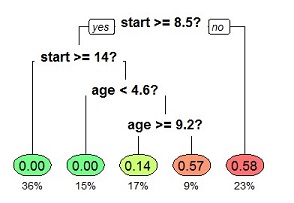
In the training phase of a decision tree, the number of points that have passed through each node is recorded in the value attribute. value is a vector of integer, where value[i] is the number of points belonging to class i that have been observed passing through the node during the training phase. For example, if three points of class index 0 and two points of class index 1 have been observed in a leaf node, the value vector of that leaf node is going to be [3, 2]. Thus, the probability for class 0 is 3/5=60%, and the probability for class 1 is 2/5=40%.
Each leaf node has a mandatory property:
valueis a vector, wherevalue[i]is the number of points belonging to classi(according to description above). Thus,value[i]/sum(value)estimates the probability for classiin the leaf.
The following example shows a decision tree with two internal nodes and three leaf nodes.
set :tree =
{
  "feature": 1,
  "threshold": 0.0,
  "left":
    {
      "feature": 0,
      "threshold": 1.0,
      "left": { "value": [4, 0] },
      "right": { "value": [1, 1] }
    },
  "right":
    {
      "value": [0, 4]
    }
};
This record can then be converted to a decision tree, using the function
rf:decisiontree(Record r) -> Decisiontree
Such a decision tree can be used for classification using
rf:dt_classify(Decisiontree dt,Vector v)->Integer
, which infers the class belonging of vector v using the decision tree dt.
In the example below, a number of different vectors are classified using :tree specified above.
select i, j,
       "class: " + rf:dt_classify(rf:decisiontree(:tree), [i,j])
  from integer i, integer j
 where i in iota(-1,1)
   and j in iota(0,2);
A number of classifier trees (a forest) can be generated using an OSQL query, such as
create function gen_forest()->Bag of Record
  as select r
       from Record r, Integer i
      where r = {
                  "feature": 1,
                  "threshold": i,
                  "left":
                    {
                      "feature": 0,
                      "threshold": 1.0,
                      "left": { "value": [4, 0] },
                      "right": { "value": [1, 1] }
                    },
                  "right":
                    {
                      "value": [0, 4]
                    }
                }
        and i in iota(-2,2);

gen_forest();
This population of trees can then be used to classify a (population of) point(s).
The example below shows how a population of trees classify the point [0,0].
select "class: " +
  rf:dt_classify(rf:decisiontree(gen_forest()), [0,0]);
Note how the prediction from each tree is shown. In Random Forest classification, the predictions of all the trees are combined.
Try classifying [0,0] using our example gen_forest():
rf:classify(rf:decisiontree(gen_forest()), [0,0]);
The predicted class of [0,0] was 1, as that class had probability 0.6 according to the generated random forest.
API
All random forest functions are listed in the OSQL API.