
TensorFlow Lite
| Module specification | |
|---|---|
| SA Engine version: | 4.13.0 (full system only) |
| Supported platforms: | Windows, Linux(x86), Raspberry Pi |
TensorFlow Lite is a mobile library for deploying neural network models on mobile, microcontrollers and other edge devices. This plugin provides an API for running TensorFlow Lite models in SA Engine.
Load the plugin
The Tensorflow Lite plugin is not a part of the base system and needs to be loaded into SA Engine. Load the plugin by running the following query:
loadsystem(startup_dir() + "../extenders/tflite","tflite.osql");
To run this code block you must be logged in and your studio instance must be started.
Download example models
This documentation uses TensorFlow Lite models that are not bundled with SA Engine. To download these models, run the following commands:
http:download_file(
    "http://assets.streamanalyze.com/tensorflow_lite_tutorial/tflite-models.s.fcz",
    {}, temp_folder() + "tflite-models.s.fcz");
sfcz:unpack(temp_folder() + "tflite-models.s.fcz",
            temp_folder() + "tflite-models", False);
To run this code block you must be logged in and your studio instance must be started.
Example 1 - A simple linear regression network
The model
In this first example we use a simple linear regression model that predicts the fuel efficiency (miles per gallon, MPG) for cars based on the vehicle's horsepower.
The model was trained and downloaded from the linear regression with one variable tutorial on the official Tensorflow site.
It takes an input tensor with a single value (horsepower) and produces a single-valued ouptput tensor (predicted miles per gallon).
The image below shows the model's training data points and resulting regression line.
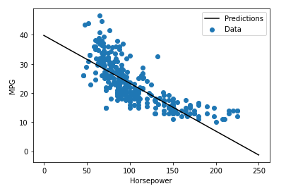
We see, for example, that for cars with around 50 horsepowers the model should predict an MPG around 30, and for cars with around 150 horsepowers the model should predict an MPG around 15.
Load the model
Load the model with tfl:read_binary_file and store the result in the tfl:model table.
set tfl:model('horsepower') =
    tfl:read_binary_file(temp_folder() +
                         "tflite-models/horsepower_model.tflite");
To run this code block you must be logged in and your studio instance must be started.
Inference
Inference is done with the function tfl:predict.
tfl:predict(Charstring name,
            Stream of Vector of Vector of Number s)
  -> Stream of Vector of Vector of Vector of Number
The string name is the name we provided in the previous step when we loaded the TFL model. The model input is a tensor (in this case only containing a single value). The input tensor is wrapped in a batch vector. You can run multiple predictions at once by putting more than one input tensor in the batch vector, but we will cover batch runs later in this tutorial. And finally the batch vector is wrapped in a stream s and passed to tfl:predict.
The output of tfl:predict is a stream, so to get the value we wrap the query in a call to extract. Run the prediction by executing the following query.
roundto(extract(tfl:predict('horsepower', streamof([[180]]))), 2);
To run this code block you must be logged in and your studio instance must be started.
The query should produce the following result.
[[[9.93]]]
This means that the linear regression model predicts that a vehicle with 180 horsepowers has a fuel efficiency of approximately 9.93 miles per gallon.
Input and output formats
As we mentioned, the input parameter s in tfl:predict is a stream of batches of input tensors , where
tfl:predict currently only supports Tensorflow Lite models with a single input tensor.
In the example the input to the horsepower model was a single-valued tensor, which we represented with a vector [180]. We only wanted to run a single prediction, so our batch only contained a single vector and the input parameter s was set to streamof([[180]]).
The output format is a stream of output batches. Each output batch is a vector of output vectors (one for each input vector ) and, since a TFL model can have multiple output tensors, each output vector
In the example above the input vector [180] produced an output vector [[9.93]] containing a single tensor [9.93] as prediction result. And since the input batch only contained one input tensor, the output vector was the only element in the output batch [[[9.93]]].
Batch predictions
As mentioned above, tfl:predict can do prediction in batches. This reduces the amount of setup and tear down the plugin needs to do compared to if the same number of predictions were carried out by sequential calls to tfl:predict.
To do a batch prediction, simply provide more than one input tensor when calling tfl:predict. The following query predicts the MPG for two vehicles with 180 and 50 horsepowers using the horsepower model.
roundto(extract(tfl:predict('horsepower', streamof([[180], [50]]))), 2);
To run this code block you must be logged in and your studio instance must be started.
Executing the query should produce the following result since now we have two output vectors in the result (with one output tensor each).
[[[9.93]], [[31.86]]]
Predictions from stream of data
We have previously used the method streamof to produce input to tfl:predict from hardcoded data. Just to show that prediction can be done on streams coming from other data sources we can simulate a regular stream of horsepowers by using the simstream function.
To run the horsepower model on a stream of simulated horsepower values we first create a function that generates a stream of values between 50 and 200 emitted every tenth of a second.
create function horsepower_stream()
  -> Stream of vector of vector of number
as select Stream of [[h]]
     from number h, number x
    where x in abs(simstream(0.1))*100
      and h = min(max(x, 50), 200)
      limit 20;
To run this code block you must be logged in and your studio instance must be started.
Now we can simply use the function as input to tfl:predict.
extract(tfl:predict('horsepower', horsepower_stream()));
To run this code block you must be logged in and your studio instance must be started.
The result should be a stream of MPG values predicted from the horsepower values produced by horsepower_stream.
[[[31.8575820922852]]]
[[[31.8575820922852]]]
[[[31.8575820922852]]]
[[[31.8575820922852]]]
[[[26.6167335510254]]]
[[[22.4122943878174]]]
[[[31.8575820922852]]]
[[[31.8575820922852]]]
[[[26.1537971496582]]]
[[[7.09315490722656]]]
...
Example 2 - Regression with a deep neural network (DNN)
In this section we will show how to make predictions with a deep neural network (DNN).
The DNN model
The model we use is a deep neural network that predicts the fuel efficiency (miles per gallon, MPG). It is similar to the model in the previous section but it takes multiple input values and has some hidden layers.
The model was trained and downloaded from the regression with a deep neural network tutorial on the official Tensorflow site.
It takes an input tensor with nine values (cylinders, displacement, horsepower, weight, acceleration, model year, Europe, Japan, and USA) and produces a single-valued ouptput tensor (miles per gallon).
Load the model
Load the model with tfl:read_binary_file and store the result in the tfl:model table.
set tfl:model('dnn_model') =
    tfl:read_binary_file(temp_folder() +
                         "tflite-models/dnn_model.tflite");
To run this code block you must be logged in and your studio instance must be started.
Inference
As described in the previous section, inference is done with the function tfl:predict. It takes the name of the model and a stream of batch inputs as input parameters.
So to use the DNN model for inference, simply run tfl:predict with the the model name and some vehicle data as input vectors.
In this example we want to predict MPG for two vehicles with the following stats:
| Car | Cylinders | Displacement | Horsepower | Weight | Acceleration | Model year | Europe | Japan | USA |
|---|---|---|---|---|---|---|---|---|---|
| #1 | 8 | 390.0 | 190.0 | 3850.0 | 8.5 | 70 | 0 | 0 | 1 |
| #2 | 8 | 360.0 | 215.0 | 4615.0 | 14.0 | 70 | 0 | 0 | 1 |
To do this we simply make a vector of stats for each car and put the vectors in a batch vector and pass it as a stream into tfl:predict.
roundto(extract(tfl:predict('dnn_model',
          streamof([[8, 390.0, 190.0, 3850.0, 8.5, 70, 0, 0, 1],
                    [8, 360.0, 215.0, 4615.0, 14.0, 70, 0, 0, 1]]))), 2);
To run this code block you must be logged in and your studio instance must be started.
The predictions should produce the following result.
[[[15.12]], [[11]]]
This means that the regression model predicts that "Car #1" has a fuel efficiency of approximately 15.12 MPG and "Car #2" has a fuel efficiency of approximately 11.0 MPG.