
Generate Simulated Audio Stream
In this part we cover how to produce a simulated audio stream. This
stream can be used as a replacement for the audio() function
used in Querying the microphone.
First we will go through the basics of harmonic sound waves. Then we'll use that to generate a sound wave for a specific frequency. Once we have that, we'll expand it to generate a sound wave of varying frequency.
Sound waves
One of the simplest harmonic sound waves is the sine wave (or sinusoid), a mathematical curve that describes a smooth periodic oscillation:
where A is the amplitude and f is the frequency (Hz).
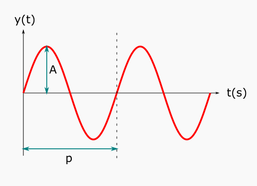
The p in the figure is the period .
Example:
sin(heartbeat(0.1))
Generating a 200 Hz Wave
A normal human ear can hear sounds in the frequency spectum around 100 Hz - 10 kHz, and some even lower or higher than that.
To generate a 200 Hz sine wave we simply plug in 200 as the frequency in Eq.(1) above.
You will not be able to hear anything when running the example below. It only produces numeric values as output and nothing gets directed to your speakers.
Example:
sin(200 * 2 * 3.1415926 * heartbeat(1/16000.0))
The value 16000 in the example above is the sampling rate - the rate at which we sample the heartbeat function.
Generating a Wave with Varying Frequency (Frequency Modulation)
A single-frequency wave is, by definition, quite monotone. Therefore we'll spice things up by varying (or modulating) the frequency of our sound wave.
The Frequency Component
Consider the following oscillation of the frequency, where is the lowest and is the highest.

Do not confuse this sine wave with the actual sound wave. This is only shows how we want the frequency component of the sound wave to vary over time.
In the figure above we have
So if we want to have a frequency that changes over time between 100-900 Hz with a period of 10 seconds, we have to rewrite Eq.(2) and substitute and A with some expression of and .
Now we can rewrite Eq.(2) as
Let us define this function as get_frequency().
Example:
create function get_frequency(Number low, Number high, Number period, Number t) -> Number
    as low + ((high - low)/2.0) * (1 + sin(2 * 3.1415926 * t / period));
The example below illustrates how the frequency will vary over time.
Example:
get_frequency(100, 900, 10, heartbeat(0.1))
Notice how the frequency oscillates between 100 Hz (low) and 900 Hz (high).
Using the Varying Frequency in the Signal
So now we have a function for the frequency. We'll refer to it as simply since all parameters except time are constants.
We cannot simply pop it into Eq.(1) since is actually a special case only valid for constant frequencies. When using frequency modulation we need to use the general equation for a sinusoid signal which is
where the integral goes from 0 to t. Note how when is constant Eq.(4) degrades to the special case which we had in Eq.(1). Therefore we need to compute the integral of our f(t) (let us call it ) and use that in Eq.(4).
By computing the integral of (Eq.(3)) between 0 and t we get
Let's define as a new function get_phase().
Example:
create function get_phase(Number low, Number high, Number period, Number t) -> Number
    as low * t + ((high - low)/2.0) * (t - cos(2 * 3.1415926 * t / period));
We use this function, with our chosen values , , and (and ), in Eq.(4) to get a signal that varies in frequency between 100-900 Hz every 10 seconds.
Let's try it in a live stream example.
Example:
select Stream of y
    from Number t, Number sr, Number y, Number phase
    where sr = 16000.0
      and t in heartbeat(1/sr)
      and phase = get_phase(100.0, 900.0, 10.0, t)
      and y = sin(2 * 3.1415926 * phase)
Creating a Simulated Version of Audio()
Now that we have a synthetic audio stream we only need to wrap it with the
appropriate interface that mimics the audio() function. In the
documentation of the audio() function we can find the signature.
> doc("audio")
"audio(Number windowsize,Number samplerate)->Stream of Vector of Number:
     ..."
We see that audio() returns a stream of vector of number, and takes the
window size (the length of each vector) and sample rate as parameters.
So to mimic this signature we wrap the entire call to our sine wave in a
winagg() function. This will provide us with a stream of vector of number.
We set the window size as an input parameter, and we also replace our fixed
sample rate sr = 16000.0 with a second input parameter. And we're done!
Example:
create function simaudio(Number windowsize, Number samplerate)
                         -> Stream of Vector of Number
    /* A simulated audio stream that varies in frequency
     between 100-900 Hz every 10 seconds. */
    as winagg(
      (select Stream of y
        from Number t, Number y, Number phase
        where t in heartbeat(1/samplerate)
          and phase = get_phase(100.0, 900.0, 10.0, t)
          and y = sin(2 * 3.1415926 * phase)),
      windowsize, windowsize);
We can test the method by simply calling it with some appropriate values for window size and sample rate.
Example:
simaudio(256, 16000)
It might be difficult to see, by only visualising the signal, how the frequency oscillates between 100-900 Hz. One can just barely make out that the sine wave becomes a bit thicker and thinner, alternating over time.
To make the variation extra clear we can use one of the first examples
from the Querying the microphone tutorial, that uses
the Fourier transform to plot the frequency of a signal over time, and
simply replace the call to audio() with a call to simaudio() and
remove the frequency filtering.
Example:
select Stream of hz
  from Number hz, Number index, Number max, Number windowSize,
       Number sampleRate, Vector of Number window
 where windowSize = 512
   and sampleRate = 16000
   and window in rfft(simaudio(windowSize,sampleRate))
   and max = max(window)
   and window[index] = max
   and hz = index * sampleRate/windowSize  * 0.5