Vision-based defect detection on Raspberry Pi using Stream Analyze Platform

Introduction

Defect detection demo summary

Defect detection is a crucial part of quality assurance in the manufacturing process. This demo uses a regular Raspberry Pi with a touchscreen to run a vision-based artificial intelligence model for defect detection in manufacturing. The model identifies defects on a manufactured part represented by a Lego build and communicates the results as visual aid to a human operator and a score to a public MQTT broker. The reason for using a Lego build instead of some specific manufactured part is to showcase the general applicability of the solution.

A screenshot of the application is shown in Figure 1.

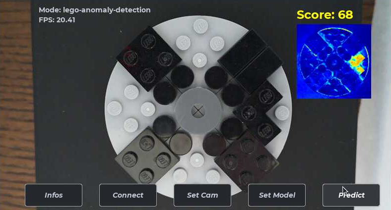
Figure 1: Defect detection application.

A complete vision pipeline containing an autoencoder was developed for this demo to provide visual feedback and a score to a manual operator. Based on the visual feedback and the score, the manual operator can determine whether any defects exists and act on objective information.

The screen shows an application that displays the camera feed, the results, and buttons for managing the camera and triggering the defect detection. The application was built using Python but the entire AI pipeline is handled by the Stream Analyze Platform.

The steps needed to develop this demo includes:

• Assembling hardware
• Data collection
• Vision pipeline design
• Model creation and training
• Application code development including embedding SA Engine into a Python application
• System performance analysis

Defect detection systems

A defect detection system is used to inspect products and detect anomalies such as broken parts, smudges, discolorations, scratches, and so forth. It feeds information to a filtering system (for example a robot arm, or in this case, a manual operator) to separate units that are not accepted fit for their intended use. Depending on the types of the products and the expected defects, various types of input can be used, including camera, laser, microphone, and so forth. This demo focuses on vision-based inputs. A typical defect detection system consists of the following components:

• A camera with appropriate resolution and frame rate.
• A computational unit to perform the AI model inference and other processes such as logging, statistics calculation, reporting to servers, networking and so forth. This demo uses a regular Raspberry Pi 4.
• Some means of delivering the units under test. This can be a conveyor belt or a manual operator that inserts the units into the test setup.
• Screen (monitor) to show information as needed, for example live feed of camera and detection result.
• Means of filtering rejected units based on AI model inference result.
• Other parts such as alarm and networking solution as needed.

Using deep learning (DL) for processing vision-based input has become popular due to its performance advantages over conventional machine vision algorithms. The next section presents some differences between the two approaches.

Conventional machine vision vs deep learning

Conventional machine vision uses rule-based algorithms and statistics. Such algorithms require expert knowledge in image processing to define rules and develop algorithms that are specific for the application domain. The conventional algorithms often consist of some detection of features and measurements followed by a series of conditional decisions aided by statistical algorithms. Developing conventional machine vision algorithms generally requires lots of time for implementation and tuning, and the resulting algorithms are often vulnerable to small changes in the domain that might render the assumptions, which the algorithms were based on, obsolete.

Since 2012, deep learning has become a popular tool in machine vision. It has shown to outperform conventional machine vision for a number of specific problems. Deep learning models can easily be trained with the appropriate dataset, without the need to specify features or rules, which require expert knowledge in image processing. Deep learning models have shown to provide higher accuracy in a number of common pattern detection problems and are generally less sensitive to variations in the domain as long as they have been trained with an appropriate dataset. The drawbacks of deep learning for machine vision is that it is mainly suitable for pattern recognition tasks, such as identifying objects or anomalies. It is also incredibly complex to analyze the workings of a deep neural network, so when a deep learning system performs poorly it it can be difficult to correct since the underlying problem is hard to deduce.

Due to the strengths and limitations of each approach, there is often an advantage to mix deep learning with conventional machine vision to achieve desired results.

Deep learning models vs mixed models

The current paradigm in the field of Edge AI focuses on designing a deep learning model to singlehandedly solve the problem to the best of its abilities. And then use embedded programming to implement the model into some processing pipeline. This can work well if the problem is limited to a pattern recognition task that deep learning solves well, like object recognition or image classification, but if the output of the deep learning model needs to be further processed, then it is often vital to incorporate conventional machine vision algorithms, like statistics and measurement algorithms, to complement the deep learning model.

So it is often necessary to use mixed models, i.e., models that incorporate both deep learning algorithms as well as conventional machine vision algorithms. This is generally done by separating the system flow into a deep learning model followed by "application code" that implements the conventional algorithms, typically in C/C++ or Python. However, using application code to implement parts of a mixed model comes with significant drawbacks such as the need for compilation, firmware updates, additional software lifecycle management to handle the application code, and it does not scale well to large fleets of devices. Also, model evolution (i.e., modifying and updating models on the device) is significantly hampered by the slow software lifecycle process, and deployments cause unwanted interruptions to production.

With the Stream Analyze platform mixed models are bundled into a single model format that can be updated and deployed to devices without the mentioned problems, making it far more versatile than the current dominating paradigm. In this demo we bundle the deep neural network (the autoencoder) with image processing operations and statistical analysis algorithms to form a single mixed model, without the need for additional application code for the analysis pipeline.

Pipeline description

The AI pipeline for this demo was implemented completely in SA Engine. SA Engine can run standalone, but for this particular demo it was convenient to embed it in a Python GUI app to get easy access to the camera interface, and to enable some interactivity into the application. The Python GUI app handles the camera input and the display to screen.

A schematic illustrating the pipeline is shown in Figure 2.

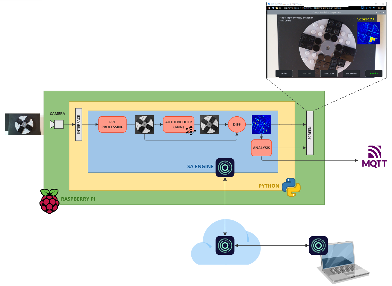
Figure 2: Quality control schematic.

The Raspberry Pi (green) has a mounted Pi Camera module 3 that takes images and passes them into a Python application (yellow). Embedded inside the Python application is SA Engine (blue). The Python application passes the images through to SA Engine for processing. In SA Engine we have the Edge AI model. The model consists of the following steps.

• PREPROCESSING: Cut out a region of the image and scale it to fit the input format of the autoencoder.
• AUTOENCODER: A deep learning model that has been trained on images of parts without any defects.
• DIFF: Difference between the autoencoder input and output.
• ANALYSIS: Statistical algorithm quantifying the level of defect.

The difference image is passed to the screen as visual aid for the operator. Also the quantified defect level is shown as a score on the screen. A high score indicate a high probability of defect, and a low score means a low probability.

The defect level is also passed as a message through MQTT to a public broker. This is to illustrate how analysis results (either intermediate or final) can be communicated over the network to entities such as monitor centers or control software.

Hardware setup

To mimic the scenario of a quality control station in an manufacturing pipeline we built a portable device which enables simple and reproducible defect detection (see Figure 3). The top of the device has room for the Raspberry Pi with a camera and touchscreen mounted. The base of the device can hold a sled on which the manufactured parts can be placed. This makes for easy insertion and removal of parts under test.

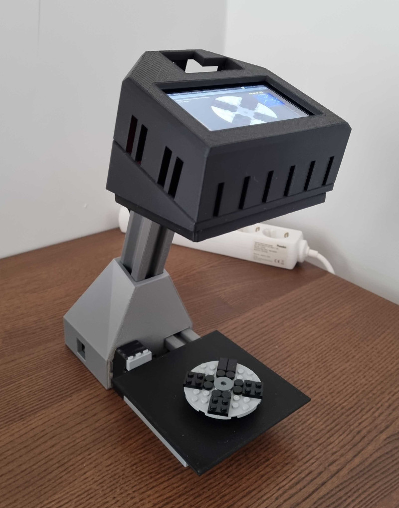
Figure 3: Quality control station.

Data set preparation

The part examined for defects is a Lego build that consists of a round light grey plate with a black cross and a dark gray center (see Figure 4). It can be rotated in any orientation around its central axis, and the black cross simulates some kind of plastic propeller-like structure that has been manufactured by molding.

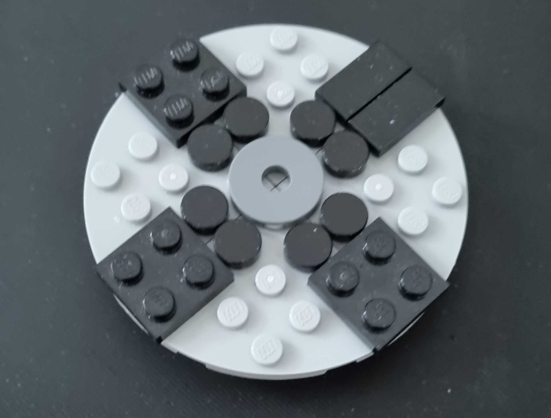
Figure 4: Example of part inspected for defects.

A defect we want to be able to detect could be plastic that has escaped the mold and produced an irregular edge. Or missing plastic, causing a dent in the mold. Or a simple miscoloration. Figure 5 shows an example of simulating a plastic leakage defect.

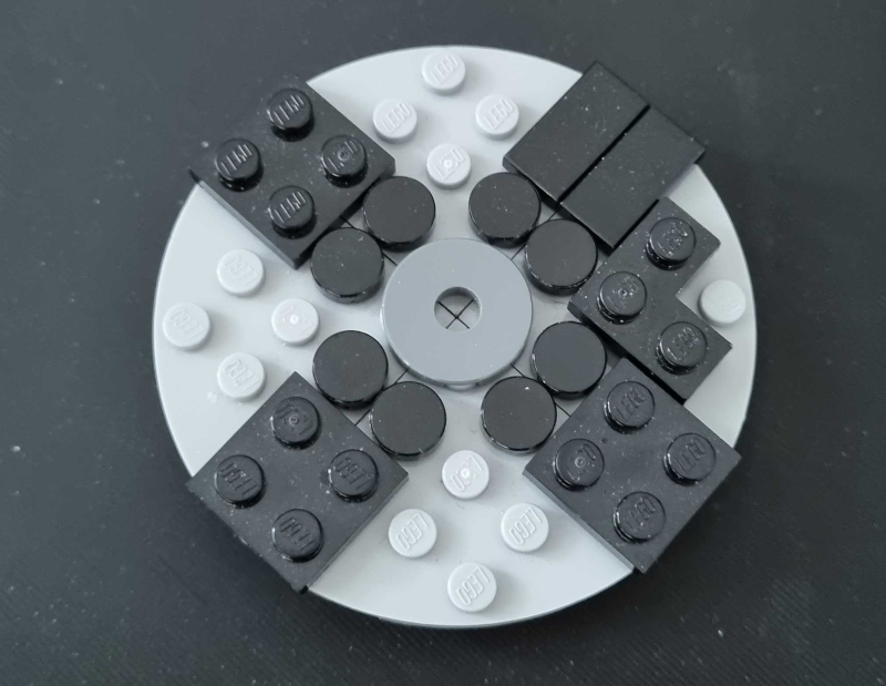
Figure 5: Example of part with defect.

The autoencoder should recognize images of ok parts. So whenever an image of an ok part is passed to the autoencoder, the output will be as similar to the input as possible. And when an image of a defective part is passed into the autoencoder, it will "disregard" the defect and output what the part would have look like if there was no defect. This facilitates to isolate any defect by taking the difference between the input image and output image from the autoencoder. The difference image will have high intensity values for the pixels in defected areas, and low intensity values for pixels in areas with no defect.

In order to train the autoencoder we needed to acquire a large set of images of the lego build. For the model to perform well the lighting conditions need to be as similar as possible to the site where the defect detection system is going run in production. Ideally for the acquisition of training images you create a fully controlled environment that can be recreated on the production site, or you even do the image acquisition on the production site.

We used the same device to collect the training data set as we used later for testing. We collected around 1200 images in fair lighting conditions that we anticipated would work well for this demo.

The images were acquired without any processing. Any preprocessing needed was done in the subsequent model training step.

Autoencoder

The autoencoder was created in Keras Python by defining the individual layers.

inputs = tf.keras.Input(shape=(128, 128, 1), name='input_layer')

encoder_net = tf.keras.Sequential(
      [
          InputLayer(input_shape=(128, 128, 1)),
          Conv2D(16, 4, strides=2, padding='same', activation=tf.nn.relu),
          Conv2D(32, 4, strides=2, padding='same', activation=tf.nn.relu),
          Conv2D(64, 4, strides=2, padding='same', activation=tf.nn.relu),
          Conv2D(128, 4, strides=2, padding='same', activation=tf.nn.relu),
          Conv2D(256, 4, strides=2, padding='same', activation=tf.nn.relu),
          Flatten(),
          Dense(encoding_dim,)
      ])

decoder_net = tf.keras.Sequential(
      [
          InputLayer(input_shape=(encoding_dim,)),
          Dense(4*4*128),
          Reshape((4, 4, 128)),
          Conv2DTranspose(128, 4, strides=2, padding='same', activation=tf.nn.relu),
          Conv2DTranspose(64, 4, strides=2, padding='same', activation=tf.nn.relu),
          Conv2DTranspose(32, 4, strides=2, padding='same', activation=tf.nn.relu),
          Conv2DTranspose(16, 4, strides=2, padding='same', activation=tf.nn.relu),
          Conv2DTranspose(1, 4, strides=2, padding='same', activation='sigmoid')
      ])

autoencoder = tf.keras.Model(inputs,decoder_net(encoder_net(inputs)))
optimizer = tf.keras.optimizers.Adam(lr = 0.0005)
autoencoder.compile(optimizer=optimizer, loss=SSIMLoss)

The autoencoder was trained on 1126 images, and then validated manually on 181 images.

After training we got a .h5 file and used a Python script to convert the network to our proprietary SANN (Stream Analyze Neural Network) representation.

OSQL model

The autoencoder is a vital part of the pipeline, but we needed a few more elements for the pipeline to be useful. We implement the pre-processing, difference operation, statistical analysis, and MQTT communication in OSQL, and bundled them together with the autoencoder into an OSQL model. By incorporating all pre-processing, postprocessing, statistical analytics, and MQTT communication into the OSQL model we have a convenient way of modifying all elements without having to restart the application.

In the following sections we describe each part of the pipeline and how they were implemented.

Preprocessing

The preprocessing step prepares the image for the autoencoder (Figure 6). It cuts out a quadratic region containing the lego disk and resizes the image to fit the autoencoder input layer. It also converts the image to grayscale since the autoencoder operates on grayscale images.

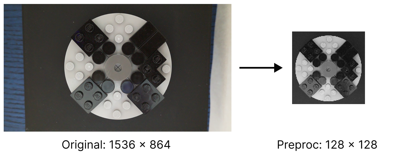
Figure 6: Preprocessing the image.

The code listing below shows the preprocessing function. Cropping, resizing, and color conversion are all part of the cv system model available in SA Engine.

create function preprocess(Array of U8 image) -> Array of U8
  /* The preprocessing step in the analysis pipeline.
     Crops the image and converts it to grayscale
     (without normalizing the intensities to full dynamic range). */
  as select preproc_im
       from Array of U8 im, Array of U8 resized_im, Array of U8 preproc_im
      where im = cv:crop(image, 50, 365, 795, 795)
        and resized_im = cv:resize(im, 128, 128)
        and preproc_im = cv:rgb2gray(resized_im);   // No normalization

Autoencoder inference

After the preprocessing step we run the image through the autoencoder. Since the autoencoder has only been trained on parts without defects, the output will show what the input would look like without defects (Figure 7).

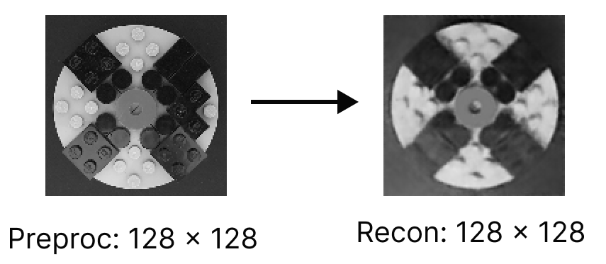
Figure 7: Autoencoder step.

The autoencoder is initialized by loading the encoder and decoder into SA Engine with sann:import(). To run the autoencoder we execute sann:classify() on both the encoder and the decoder. The following code illustrates the inference step of the pipeline.

sann:import("AE_LEGO_QC_encoder",
            models:folder("lego-anomaly-detection") + "autoencoder/AE_LEGO_QC_encoder");
sann:import("AE_LEGO_QC_decoder",
            models:folder("lego-anomaly-detection") + "autoencoder/AE_LEGO_QC_decoder");

create function run_encoder(Array image) -> Array
  as sann:classify(sann:named("AE_LEGO_QC_encoder"), image);

create function run_decoder(Array encoded_image) -> Array
  as sann:classify(sann:named("AE_LEGO_QC_decoder"), encoded_image);

create function run_inference(Array image) -> Array
  as run_decoder(run_encoder(image));

create function recon(Array of U8 im) -> Array of U8
  as select array("U8", recon)
       from Array of F64 gray_imi_f64, Array of F64 gray_imi_f64_norm,
            Array of F32 recon_imi, Array of F32 recon
      where gray_imi_f64 = array("F64", im)
        and gray_imi_f64_norm = gray_imi_f64 / 255
        and recon_imi = reshape(run_inference(gray_imi_f64_norm), [128,128])
        and recon = recon_imi * 255;

The main function here is recon(). It takes a graylevel U8 (unsigned 8-bit) image and converts it to 64-bit floating point (L19), normalizes it to values between 0.0-1.0 (L20), and runs the autoencoder inference on the normalized image (L21). The output from the autoencoder is a flat array, so we reshape the output to 128x128 and multiply all values by 255 to get a range between 0-255 (L22). Finally we convert the datatype to unsigned 8-bit before returning the result (L16).

Image difference and statistical analysis

The autoencoder outputs an image depicting how the Lego build would look if there were no defects. So we take the difference of the image passed to the autoencoder, and the output from the autoencoder (Figure 8).

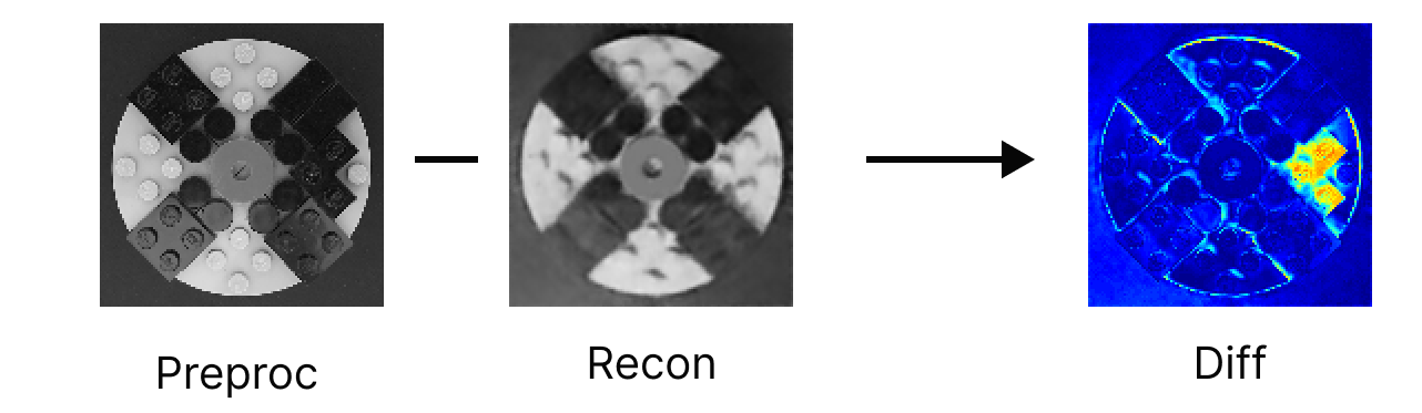
Figure 8: Difference step.

For the statistical analysis we use Otsu's method (Wikipedia) as a measure of the level of defect in the image. Otsu's method looks at the histogram of an image and finds the threshold value that best separates two normal distributions in the histogram.

In our case, if there is no (or low) difference between the two images, i.e., if there is no defect in the image, then the histogram will have one large distribution of values near zero and Otsu's method will assume the two normal distributions overlap and thus generate a low threshold somewhere in the middle of that distribution (see Figure 9(a)). But if there is a defect present in the image, the histogram will have one distribution near zero and another distribution of values higher up in the histogram representing the pixels where the images differ, i.e., where we have the defect. In this case Otsu's method will identify the two distributions and produce a threshold somewhere higher up on the scale about halfway between the two distributions. So images with defects will therefore result in higher Otsu thresholds than images without defects (see Figure 9(b)).

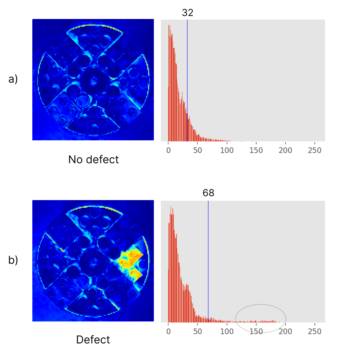
Figure 9: Analysis step.

The following code illustrates the difference operator and the statistical analysis using Otsu's method.

create function colorize(Array of U8 diff_im) -> Array of U8
  /* Colorize the difference image and send it out on a flow. */
  as select diff_im_col
       from Array of U8 diff_im_col
      where diff_im_col = emit_on_flow(cv:gray2rgb(diff_im, cv:const:colormap_jet()), "diff_im_col");

create function compute_otsu(Array of U8 orig_im) -> Integer
  /* The "main" analysis pipeline.
     Strings together all parts of the analysis and returns the Otsu threshold
     result as string. */
  as select threshold
       from Array of U8 recon_im,
            Array of U8 diff_im,
            Array of U8 diff_im_col,
            Integer threshold
      where recon_im = recon(orig_im)     // Reconstructed image (w/o normalization)
        and diff_im = emit_on_flow(array("U8", abs(array("F64", orig_im) .- array("F64", recon_im))),
                                   "diff_im")
        and diff_im_col = colorize(diff_im)
        and threshold = emit_on_flow(cv:otsu_binarization(diff_im), "threshold");

The main function here is compute_otsu() which handles the analysis. It takes the preprocessed image as input and outputs the threshold value, which we use as defect level. The function calls recon() to apply the autoencoder on the preprocessed image (L16). The output from the autoencoder and the preprocessed image are both converted to 64-bit float and subtracted from each other (L17-18). The function emit_on_flow() simply publish the result on a stream for debugging and visualization purposes. The difference image is converted from grayscale to color using the colorize() function (L19). Otsu binarization is computed on the graylevel diff image to produce the threshold we use as defect level (L20), and finally the threshold from the analysis is returned from the compute_otsu() function (L11).

Put it all together

Now we have covered the different parts of the OSQL model. Now we simply need to put it all together with a high-level function that can be triggered from the application.

create function analyze(Array of U8 im) -> Charstring
  /* External API function. */
  as select stringify(threshold)
       from integer threshold, Record score_rec
      where threshold = compute_otsu(preprocess(im))
        and score_rec = emit_on_flow(json:stringify({"score": threshold}), "analysis-result");

The function takes the original image that will be passed in straight from the camera via Python to OSQL (L1). It calls the preprocessing and passes the result to the analysis function (L5). The threshold is emitted as a JSON on a stream to be picked up by the MQTT publisher thread (L6). Finally the threshold value is converted to a string and returned as result (L3). This result will be picked up by the Python application and passed on to the screen.

Application development

Application overview

The Python application embedding SA Engine is designed to be a simple interface for the manual operator to run the defect detection pipeline.

main.py

import numpy as np
import sa
import settings
#...

def main(argv):
    # Init camera
    cam = CamHandler()

    # Init model
    model_handler = ModelHandler("lego-anomaly-detection")
    model_handler.setup()

    # Subscribe to diff image stream (for visualization)
    sa.SAEngineModel().run_diff_stream()

    # Setup MQTT client
    sa.SAEngineModel().setup_mqtt(settings.MQTT_BROKER, settings.MQTT_TOPIC)

    # Setup GUI
    #...

    # Setup camera capture
    #...

    # Start loop
    while running:

        # Timing control
        #...

        # Refresh cam image
        #...

        # Update diff image
        current_diff_image: np.array = sa.SAEngineModel().current_diff_image()
        if current_diff_image is not None:
            gui.update_diff_image(current_diff_image)
            
        # Display cam image
        #...
        
        # Process GUI events
        running = gui.process_events(...)

        # Update GUI
        #...

    # Cleanup
    #...


if __name__ == '__main__':
    main(sys.argv)

We start by importing important packages. For example sa handles interactions with SA Engine (L2), and settings contains some configurations for connecting to server and MQTT (L3). Then we setup the model handler and load the OSQL model (L12). The model handler is a middle layer that handles the interaction with SA Engine through the sa package. After the model has been initiated we start the difference image stream (L15). The difference image stream provides frames that will be displayed on screen as part of the result. Then we start the MQTT stream that publishes the defect levels to a public MQTT broker (L18).

Once the setup is done we move into the main loop. Here we start by handling the timing and live video feed from the camera. Then we extract the diff image result (L36) and update the diff image on screen (L38). And finally we process any GUI events, like triggering the defect detection pipeline or connecting to server (L44).

We'll break down each of these important steps in the following sections.

Start SA Engine

At the top of main.py we import sa.py which handles all interactions with SA Engine. We will cover sa.py more in depth in the following sections, but at this stage it is important to note that sa.py imports sa_python which is the Python embedding for SA Engine. This starts an embedded instance of SA Engine which is callable from within Python.

sa.py

import os
import threading
import time
import sa_python as sa_engine
import numpy as np
#...

You can read more about the Python embedding in the SA Engine Python Interfaces.

Load the OSQL model

In the setup section of main.py we call the model handler to setup the OSQL model.

main.py

#...

    # Init model
    model_handler = ModelHandler("lego-anomaly-detection")
    model_handler.setup()

#...

In our model handler we have some helper functions to check to see if the model is available and to load the model.

modelhandler.py

#...

class ModelHandler:
    def __init__(self, model_name: str):
        self.model_name: str = model_name
    
    def setup(self) -> bool:
        self.modelLoad(self.model_name)

    def modelAvailable(self) -> bool:
        return sa.SAEngineModel().is_model_loaded(self.model_name)

    def modelLoad(self, modelName: str):
        if not self.modelAvailable():
            sa.SAEngineModel().load_model(modelName)
            sa.SAEngineModel().wait_for_model(modelName)
        return None

#...

The sa package contains a singleton object SAEngineModel() that controls all interactions with SA Engine.

sa.py

#...

class SAEngineModel:
    _instance = None
    _lock = threading.Lock()

    #...

    def __new__(cls):
        if cls._instance is None:
            with cls._lock:
                # Another thread could have created the instance
                # before we acquired the lock. So check that the
                # instance is still nonexistent.
                if not cls._instance:
                    cls._instance = super().__new__(cls)
                    cls._instance.sa = sa_engine.connect("")
                    print("SA Engine activated")
        return cls._instance

    def query(self, query_text):
        return [x for x in self.sa.query(query_text)]

    def call(self, *args, **kwargs):
        return [x for x in self.sa.call(*args, **kwargs)]

    #...

    def load_model(self, name: str) -> bool:
        return self.query(f"models:load('{name}');") != [0]

    def is_model_loaded(self, name: str) -> bool:
        return self.query(f"count(select m from charstring m where m in models:loaded() and like(m, '{name}*'));") != [0]

    def wait_for_model(self, name: str):
        if not self.is_model_loaded(name):
            print(f"Waiting for model '{name}' to load")
            time.sleep(0.1)
        while not self.is_model_loaded(name):
            time.sleep(0.1)

        print("Using:", self.query(f"select m from charstring m where m in models:loaded() and like(m, '{name}*');"))

#...

The function __new__() handles all references to the singleton. So whenever SAEngineModel() is called, it returns the singleton object. If there is no instance of the singleton, it creates a new instance (L16) and connects it to SA Engine (L17). The singleton keeps the SA Engine connection in a member object called sa. This enables us to send queries to SA Engine by calling sa.query(), which we wrap in a function named query() (L21-22). We can also execute functions in SA Engine by calling sa.call(), which we wrap in another function named call() (L24-25).

We define the functions load_model(), is_model_loaded(), and wait_for_model() as sending queries to SA Engine through the query() function.

load_model() simply sends the OSQL query models:load('name'), where name is the name of the model (L30).

is_model_loaded() sends an OSQL query that returns the number models that are loaded with the matching name. Then the python function checks that the query result is not zero (L33).

wait_for_model() checks if the model is loaded, and if it is not, then the function enters a simple waiting loop that exits only when the model is loaded.

Start diff image stream

Now that the model is loaded it is time to start the stream of diff images.

main.py

#...

    # Subscribe to diff image stream (for visualization)
    sa.SAEngineModel().run_diff_stream()

#...

We do this by simply calling the function run_diff_stream() in the SAEngineModel().

sa.py

#...

class SAEngineModel:
    #...

    _diff_image: np.array = None

    #...

    def do_run_diff_stream(self):
        for x in self.sa.query("select x from Object x where x in subscribe('diff_im_col')"):
            self._diff_image = x
    
    def run_diff_stream(self):
        x = threading.Thread(target=self.do_run_diff_stream, daemon=True)
        x.start()

#...

The run_diff_stream() function starts a separate thread (L15-16) that listens to the diff image stream (L11) and stores each new diff image in a member object _diff_image (L12). The OSQL Array representation memory structure is fully compatible with np.array, so there is no overhead in the type conversion between OSQL and NumPy.

We recall from the OSQL code in the Image difference and statistical analysis section that we had the OSQL function colorize().

create function colorize(Array of U8 diff_im) -> Array of U8
  /* Colorize the difference image and send it out on a flow. */
  as select diff_im_col
       from Array of U8 diff_im_col
      where diff_im_col = emit_on_flow(cv:gray2rgb(diff_im, cv:const:colormap_jet()), "diff_im_col");

It takes the graylevel difference image and use cv:gray2rgb() with a specific color map to create a colorized version of the diff image that emphasize the defect areas. It also use the function emit_on_flow() to send the result out on the diff_im_col stream, which we subscribe to in the do_run_diff_stream() python function above (L11).

So whenever a new color diff image is produced by the OSQL function colorize(), it is placed on the stream diff_im_col, and automatically picked up by the function do_run_diff_stream() and saved to SAEngineModel()._diff_image, which will later be accessed by the main loop in the Python application.

Start MQTT stream

The final setup step is to start publishing the MQTT stream to a public MQTT broker.

main.py

#...

    # Setup MQTT client
    sa.SAEngineModel().setup_mqtt(settings.MQTT_BROKER, settings.MQTT_TOPIC)

#...

We do this by calling the setup_mqtt() function in SAEngineModel() with some configuration parameters from the settings.

settings.py

#...

MQTT_BROKER = "tcp://test.mosquitto.org:1883"
MQTT_TOPIC = "mqtt:sa-demo/metrics"

#...

We use a publicly available mosquitto broker on the topic sa-demo/metrics.

We set up the MQTT stream by calling SAEngineModel().setup_mqtt() with configuration strings from settings.py.

sa.py

#...

    def do_publish_flow(self):
        print("started do_publish_flow", self._mqtt_channel)
        self.call("publish_flow","analysis-result", self._mqtt_channel)

    def setup_mqtt(self, broker, channel):
        self.query("loadsystem(startup_dir()+'../extenders/sa.mqtt','mqtt.osql');")
        self.query("models:load('mqtt-output')")
        self.call("register_mqtt_client", broker)
        self._mqtt_channel = channel
        x = threading.Thread(target=self.do_publish_flow)
        x.start()

#...

The function setup_mqtt() loads the MQTT extender (L8), loads a MQTT model for publishing data to the broker (L9), registers the MQTT client in SA Engine (L10), stores the channel name (L11), and starts a separate thread (L12-13) that publishes the stream analysis-result to the channel (L5).

The OSQL model that handles the MQTT communication contains the following three functions.

create function register_mqtt_client(charstring broker) -> Charstring
  as mqtt:register_client("mqtt",
                          { "qos": 1,
                            "connection": broker,
                            "clientid": "client" + sha256(ntoa(rand(10e16))) });

create function send_data(record data, charstring channel) -> stream
  as select publish(data_s, channel)
       from stream of record data_s
      where data_s = streamof(data);

create function publish_flow(charstring flow, charstring channel) -> stream
  as select send_data(r, channel)
       from Record r 
      where r in subscribe(flow);

We will not go into any details about how MQTT communication is done in SA Engine. For a detailed explanation of how to use MQTT with SA Engine we refer to the MQTT module documentation.

So now whenever a new result is published on the stream analysis-result (see Put it all together), the result is published to the public MQTT broker.

Trigger analysis pipeline

The analysis pipeline is triggered by pressing the "Predict" button in the application GUI (Figure 10).

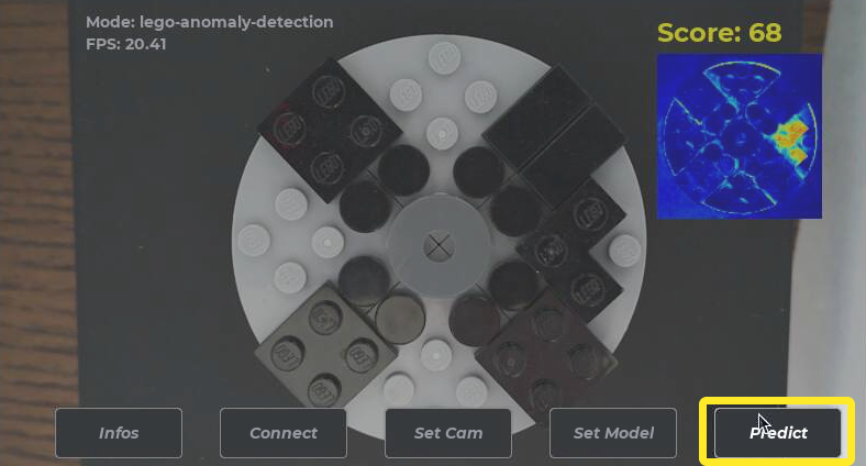
Figure 10: The predict button triggers the analysis pipeline.

This is handled in the process_events() function in the GUI handler, which is called from the main loop in the application.

pygamehandler.py

#...

class PyGameGUIClass:
    #...

    def process_events(self, npix: NeoPixelHandler, cam: CamHandler, model_handler: ModelHandler) -> bool:
        #...

        if event.ui_element == self.button_predict:
            capimg = cam.takePhoto(npix)
            result = model_handler.modelpredict(capimg)
            self.displayResult(result)

#...

When the predict button is pressed, the GUI handler extracts an image frame from the camera feed (L10) passes the frame to the modelpredict() function in the model handler (L11). It also displays the result (the defect level) as text on the screen (L12).

modelhandler.py

#...

class ModelHandler:
    #...

    def modelpredict(self, image: np.ndarray) -> str:
        result: str = ""
        if not self.modelAvailable():
            print("Error running prediction: OSQL model not loaded")
            result = "<no model>"
        else:
            print("Running inference")
            result = sa.SAEngineModel().call("analyze", image)[0]
        return result

#...

The modelpredict() function in the model handler ensures that a model is available (L8) and calls the OSQL analyze() function (see Put it all together) with the image frame as input (L13). The result is the defect level score which is returned as a string to the GUI handler, which displays the score on the screen (Figure 11).

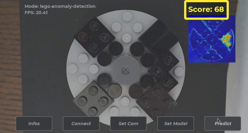
Figure 11: The defect level score displayed on the screen.

Display diff image

In the section Start diff image stream we showed how the SAEngineModel() was set up to listen to the OSQL stream diff_im_col, and save all new objects (images) on that stream to a member named _diff_image.

sa.py

#...

class SAEngineModel:
    #...

    _diff_image: np.array = None

    def current_diff_image(self) -> np.array:
        return self._diff_image

#...

So whenever the analysis pipeline is triggered, a new diff image will be stored in the _diff_image object in SAEngineModel().

We also recall from Application overview that the main loop reads the diff image from SAEngineModel() and passes it on to the GUI handler to display it on the screen.

main.py

#...

    while running:
        #...

        # Update diff image
        current_diff_image: np.array = sa.SAEngineModel().current_diff_image()
        if current_diff_image is not None:
            gui.update_diff_image(np.rot90(np.flipud(current_diff_image)))

#...

So whenever the predict button is pressed, the screen will be automatically updated with the new diff image from the analysis pipeline (Figure 12).

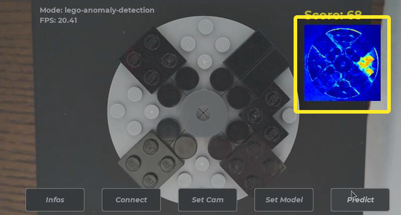
Figure 12: The diff image displayed on the screen.

Publish result to MQTT broker

In the section Start MQTT stream we set up the entire pipeline for the MQTT communication. We also started a thread that publishes any new object in the stream analysis-result to the public MQTT broker. And we recall from the Put it all together section that the analyze() OSQL function publishes a JSON containing the defect level score to the analysis-result stream.

create function analyze(Array of U8 im) -> Charstring
  /* External API function. */
  as select stringify(threshold)
       from integer threshold, Record score_rec
      where threshold = compute_otsu(preprocess(im))
        and score_rec = emit_on_flow(json:stringify({"score": threshold}), "analysis-result");

So whenever the predict button is pressed, the analyze() OSQL function is called, and the defect level result score from the analysis is published to the public MQTT broker.