Streams

One important feature of OSQL is to enable processing functions and filters over streams. In the simplest case is is an expression returning a stream.

The function heartbeat(Real pace)->Stream of Real returns an infinite stream of numbers representing the time elapsed from its start every pace seconds.

Example:

heartbeat(0.5)

The function heartbeat() is a stream generator, i.e. a function that returns a stream as an object. When you enter a stream object to the REPL it will run the stream to extract and display stream element as in the example above.

The query is an example of a continuous query (CQ) since it continuously produces objects until you explicitly stop it.

The stream generator diota(pace,l,u) returns a finite stream of the integers between l and u with pace delays in-between.

Example:

diota(0.5,1,5)

A function taking a stream as argument to produce another stream as result is called a stream function. For example, the stream function first_n(Stream s,Real n)->Stream returns a finite stream of the n first elements in s.

Example:

first_n(heartbeat(0.125),5)

The stream function timeout(s,t) runs the stream s for t seconds.

Example:

timeout(heartbeat(0.125),1.1)

The stream function skip(s,n) skips the n first elements in the stream s.

Example:

skip(heartbeat(1),1)

The stream function changed(s) returns a stream where successive duplicated elements have been removed.

Example: The duplicated elements in the stream floor(heartbeat(0.25)*2.5) have been eliminated in this query:

select changed(floor(heartbeat(0.25)*2.5)) limit 7

Stream elements are enumerated starting with number 1. The stream function section(s,b,e) returns a stream of the elements in stream s starting with element number b and ending with element number e.

section(heartbeat(0.125),3,5)

Calls to the stateful function extract(Stream s)->Bag of Object in expressions run s to extract the elements in s. The extracted elements can then be used as a regular bag in set queries by using the in operator.

Example: The following set query continuously returns sine values extracted from the heartbeat stream:

select sin(x)
  from Real x
 where x in extract(diota(0.5,1,5))

Note

The in operator can be applied directly on a stream s as well, but this will be deprecated. Thus the legacy notation e in s is the same as e in extract(s). For clarity it is recommended to use the format e in extract(s) to indicate the side effect of running s to extract its elements.

Synthetic streams

Synthetic stream generators are functions returning streams whose elements are generated by some algorithm rather than originating in some physical measurements. In the documentation synthetic streams are used for illustrating the behavior of the system. They are furthermore very useful for generating simulated data streams to test models without accessing sensors and other external data sources.

A trivial example of a synthetic stream generator is the function siota(Integer l, Integer u)->Stream of Integer that generates a finite stream of integers between l and u. It is used in throughout the documentation to produce simple predictable streams that illustrate the behavior of other stream functions.

Similarly, the stream generator diota(Real pace, Integer l, Integer u)->Stream of Integer returns a finite stream of integers between l and u with a delay of pace in-between produced elements.

Example: This query generates a finite real-time sine wave:

//plot: Line plot
sin(diota(0.01,1,100)*3.14/50)

The stream generator heartbeat(Real pace)->Stream of Real is an important built-in synthetic stream generator that can be used for defining other real-time stream generators.

Example: This stream generator function returns a real-time infinite sine wave:

create function rsin(Real pace, Real multiplier) -> Stream of Real
  as sin(heartbeat(pace)*multiplier)

Let's try it:

//plot: Line plot
rsin(0.01,10)

Exercise

Vary the parameters of rsin() and see what happens.

In general, the built-in library of trigonometric functions is very useful for generating synthetic streams. The system function simstream(Number pace) is such a synthetic stream generator that returns a simulated stream of numbers with given pace based on sine.

Example:

//plot: Line plot
simstream(0.1)

It is defined as simsig(heartbeat(pace)), thus calling the function simsig(x) each x seconds after its start at the given pace. This is an example of how to generate a synthetic stream.

Exercise

Inspect the definitions of simstream() and simsig() to see how they are defined.

The stream generator randstream(Real l, Real u)->Stream of Real generates a stream of random numbers between l and u.

Example:

//plot: Scatter plot
select randstream(0,1)
 limit 1000

The guide Generate simulated audio shows how to generate synthetic audio streams using trigonometric functions.

Select stream queries

A select stream query produces a new stream where elements fulfilling user defined conditions are filtered out. For example, the following CQ filters out the stream elements of simstream(0.1) larger than 1 visualized as a line plot:

//plot: Line plot
select Stream of x
  from Real x
 where x in extract(simstream(0.01))
   and x > 1

The CQ generates a new stream of the selected stream elements. Notice how the result stream pauses (slows down) once in a while when when elements less than 1 are produced by simstream(0.01).

Exercise

Try running:

select Stream of x
  from Real x
 where x in extract(heartbeat(0.5))
   and x < 1

Why does it stop?

You can define new stream functions as select stream queries.

Example: This stream function computes a stream of the square roots of the elements in its argument stream s:

create function sqrt_stream(Stream of Integer s) -> Stream of Real
  as select Stream of sqrt(e)
       from Integer e
      where e in extract(s)

sqrt_stream(diota(0.5,1,5))

Several objects can be grouped together in select stream queries producing streams of tuples.

Example:

select Stream of e,e*10
  from Integer e
 where e in extract(diota(0.5,1,5))

You can define stream functions producing streams of tuples.

Example:

create function mult_stream(Stream of Integer s, Integer i)
                          -> Stream of (Integer,Integer)
  as select Stream of e,e*i
       from Integer e
      where e in extract(s)

mult_stream(diota(0.5,1,5),10)

Stream windows

It is often necessary to operate on streams of finite sections of the latest elements of a stream, called stream windows, e.g. a stream of the latest 10 elements in an infinite stream. Windows are represented as vectors. There are several built-in functions for forming such streams of windows.

Tumbling and sliding windows

In general the function winagg(s, sz, str) forms a stream of windows over a stream s where each window has size sz elements. The third parameter str is called the stride and defines how many stream elements the window moves forward over the stream.

Example:

winagg(heartbeat(0.5),2,2)

In the example above the size and the stride are both 2, meaning that once a window of 2 elements is produced a new one is started to be formed. This is called a tumbling window.

If the stride is smaller than the size, new overlapping windows will be produced more often. This is called a sliding window.

Example:

winagg(heartbeat(0.5),2,1)

Exercise

Run query returning sliding window over heartbeat(0.5) with size 4 and stride 2.

Bar plots can be used for running visualizations of numerical windows.

Example:

//plot: Bar plot
winagg(sin(heartbeat(0.1)*5),10,2)

The query produces a stream of vectors (i.e. windows) by collecting into the vectors 10 elements at the time from the stream sin(heartbeat(0.1)*5) slided with stride 2.

Since heartbeat(0.1) produces a number 10 times per second and the windows contain 10 elements displayed 10/2=5 times, the result from the expression is a stream of vectors produced once per second, i.e. with pace 5 HZ.

Running aggregation

Since streams can be infinite, the computation of aggregated values over streams works differently from applying aggregate functions on bags, vectors or arrays, for which a single value is aggregated over all elements in the collection.

This is not possible for infinite collections. For example, summing all values in the stream heartbeat(0.5) would not be computable since heartbeat(0.5) is infinite and a regular application of sum would never return.

Therefore, when regular aggregate functions are applied on streams, they are applied on each element in the stream. This is called running aggregation.

Example: The aggregate function sum is applied on the vectors representing tumbling windows of size 2 in the heartbeat(0.5) stream:

sum(winagg(heartbeat(0.5),2,2))

Moving average

A common way to reduce noisy signals is to form the moving average of sliding or tumbling windows over a stream of measurements by computing the average avg(w) for each window w.

Example:

//plot: Line plot
avg(winagg(simstream(0.01),10,5))

Exercise

As an alternative, try using median() instead of avg().

This CQ returns the moving averages larger than 0.7 of windows of simstream(0.01):

//plot: Line plot
select Stream of x
  from Real x
 where x in extract(avg(winagg(simstream(0.01),5,5)))
   and x > 0.7

Here you will notice rather long pauses.

Streamed reduce

The reduce function can also be used for streams. Since streams are continuously extended sequences that can be infinite, it is not possible to compute a single aggregated values for a stream as for other collections. Furthermore, since data stream elements can be visited only once, a data stream reducer must be one-pass. Instead, the result of $reduce(S,r)$ for a stream $S$ is a new stream $R$ of running aggregations where a new element in $R$ is returned after each call to the reducer $r$.

By contrast, for other collections the reducer returns a single total aggregation for the whole collection.

Simple streamed reduce

In simple streamed reduce the function $reduce(S,r)$ takes a stream $S$ with elements $e_i$, and the binary reducer function $r(a,e_i)$ as arguments. It returns a new reduced stream $R$ with elements $f_i$ defined as follows:

$a_1 = e_1 \newline a_i = r(a_{i-1},e_i), i > 1$

The accumulator $a_i$ is initially assigned to the first element $e_1$ in $S$. The reducer $r$ is called starting with element $e_2$ in $S$. Each time it is called a new accumulated value $a_i$ is computed from a new element $a_i$ of the transformed result stream $R$. The accumulator $a$ must be of the same type as the elements $e_i$.

Example: The following expression returns the running sum of the elements in the stream diota(0.1,1,5).

reduce(diota(0.5,1,5),'+')

Analogous to simple reduce over regular collections, some simple running aggregations of can also be defined by simple streamed reduce.

Example: The following expression returns the running maximum of the elements in the stream sin(diota(0.5,1,5)).

reduce(sin(diota(0.5,1,5)),'max')

The running minimum can be defined analogously.

note

Unlike reduce over regular collection the order in which the reducer is applied is the same as the order in which the elements in $S$ are received.

Parameterized streamed reduction

As for regular collections many aggregate functions require several accumulators, which are provided as extra parameters to the reducer function. The same reducers as those used for total aggregation can also be used for defining running aggregations over streams.

Example: The mean1_reducer function can be used for defining the running average of a stream of numbers.

create function rmean1(Stream of Number s) -> Stream
  as select Stream of sum/count
       from Integer count, Real sum
      where (count, sum) in extract(reduce(s, 'mean1_reducer', 0, 0.0))

Test it:

rmean1(diota(0.5,1,5))

While regular aggregations can be multi-pass, streamed aggregations must be one pass.

Example: The function variance2_reducer can be used for a numerically stable running standard deviation defined as follows.

create function rvariance2(Stream of Number ns) -> Real
   as select s/(cnt - 1)
        from Integer cnt, Real m, Real s
       where (cnt, m, s) in extract(reduce(ns, 'variance2_reducer', 0, 0, 0))

Test it:

rvariance2(stream 1,2,3,4,5)

Streamed reduction elements

For streamed reduction it is possible to include in the result not only running aggregations, but also computations over individual incoming stream elements $e_i$. This allows to collect running statistics combined with incoming stream elements.

Example: For a given stream $S$ with numeric elements $e_i$ we define a stream $meanpairs(S)$ producing a new stream with elements being vectors $[e_i, avg(e_1,...,e_i)]$.

The reducer will be:

create function meanpairs_reducer(Number e0, Number cnt, Number sum, Number e)
                        -> (Number next_e, Integer next_cnt, Integer next_sum)
  as select e,       -- the element (e0 ignored)
            cnt + 1, -- the count
            sum + e  -- the sum

The stream aggregate function meanpairs will have the following definition.

create function meanpairs(Stream of Number s) -> Stream 
  as select Stream of [e, sum/cnt]
       from Number e, Number sum, Integer cnt
      where (e, cnt, sum) in reduce(s, 'meanpairs_reducer', 0,0,0);

Test it:

meanpairs(stream 1,4,3,5,2)

Time stamped streams

A time stamped stream is a stream of time stamped elements.

The function ts_simstream(pace) produces a synthetic stream of numbers where each element is time stamped with the wall time when it was produced. This is called a time stamped stream.

Example:

//plot: Line plot
ts_simstream(0.01)

info

Notice that the X-labels indicate the times when each element was produced. If you wait a while you will see how the stream start scrolling to the left.

Time stamped streams can be defined by time stamping the elements x of a stream's result by calling the function ts(x). For example, the following query returns the same timestamped simulated stream of numbers as ts_simstream(0.01):

//plot: Line plot
select Stream of ts(x)
  from Real x
 where x in extract(simstream(0.01))

In general, the function ts(x) time stamps any kind of object. It returns a time stamped object having the value x (see Time).

Exercise

Visualize the four first elements of the time stamped stream as text.

The function sample_stream(x, pace) returns an infinite stream of the expression x evaluated every pace seconds, for example:

sample_stream("Hello stream",1)

The following CQ returns a visualized stream of time stamped random numbers:

//plot: Scatter plot
sample_stream(ts(rand(100)),0.1)

Time stamped windows

A time stamped window is a time stamped vector representing a window in a time stamped stream.

One can time stamp any object using the ts(x) function. Therefore, calling ts(s) for a stream of windows s produces a stream of time stamped windows.

Example: The following query produces a stream of time stamped sliding windows each having 4 elements with 50% overlap:

ts(winagg(heartbeat(0.25),4,2))

Individual stream elements e in windows can also be time stamped using ts(e).

Example:

winagg(ts(heartbeat(0.25)),2,2)

Exercise

Time stamp both elements and windows in the query above. How does the time stamp of each window relate to the time stamps of its elements?

Temporal windows

The kind of windows discussed so far are called counting windows in that they produce window vectors based on counting the incoming stream elements. This is a very efficient and simple method to form windows, e.g. for continuously computing statistics over windows of arriving data, as the moving average above. It works particular well if the elements arrive at a constant pace.

If the elements arrive irregularly one may need to form temporal windows whose sizes are based on elements arriving during a time period rather than on the number of arriving elements as for counting windows.

Temporal windows are formed with the function twinagg(ts, size, stride) that takes a timestamped stream of objects as input and produces a time stamped stream of vectors of objects as result. The parameters size and stride are here measured in seconds rather than number of elements as winagg().

Example:

select tv
  from Timeval of Vector of Real tv
 where tv in extract(twinagg(ts_simstream(0.01),0.5,0.5))
 limit 10

The following query computes the mean and median of simstream with pace 100HZ each 1/2 second:

//plot: Line plot
select avg(v), median(v)
  from Timeval of Vector of Real tv, Vector of Real v
 where tv in extract(twinagg(ts_simstream(0.01),0.5,0.5))
   and v = value(tv)
 limit 10

Notice that you can apply any Vector function on v.

Bus streams

It is common that several streams from a source are duplexed into a single bus stream whose element are pairs (id,value) representing the latest value observed for a sensor identified by id:

Example: The following stream :s simulates a bus stream for three sensors with identifiers S0, S1, and S2.

set :s1 = (select Stream of 'S'||mod(i,3), i*10
             from Integer i
            where i in range(12))

:s1

We use the term signal to denote labels of sensors. Selecting the observations in a bus stream for one signal can be done with a simple select stream query.

Example: This query returns a stream of readings for signal 'S1':

select Stream of v
  from Integer v
 where ('S1',v) in extract(:s1)

Usually computations are made from more than one signal in a bus stream. The function pivot_bus(Vector keys, Stream s)->Stream of Vector produces a stream of vectors of the latest readings from the signals keys in the bus stream s. Such a stream of vectors is called a signal stream. The function pivots a bus stream into a signal stream.

If $[S_1,...,S_k]$ are the signals in keys, the elements in each signal stream will be vectors $[V_1,...,V_k]$ where $V_i$ is the latest value of signal $S_i$.

Example: This query returns a signal stream of the readings for signals 'L0' and 'L1':

pivot_bus(['S0','S1'],:s1)

Notice that first element of the signal stream is [null,10]. The reason is that the first element in :s1 is the pair ('S1',10) indicating that signal S1 has the value 10. At that point signal S0 is unknown.

A common case is to provide default defaults for missing signal values. The function defaults(Vector v, Vector d) replaces unknown values in v with the corresponding element in d.

Example::

defaults([null,10,null],[1,2,3])

We can use defaults to replace unknown values in each signal stream vector.

Example:

defaults(pivot_bus(['S0','S1'],:s1),[0,1])

Combining streams

There are a number of stream function to combine several streams. They are useful if you are working with streams of several signals and would like to combine and compare them.

Merging streams

The function merge(Vector of Stream vs)->Stream creates a new stream from the streams in vs. The elements of the merged stream are taken from each of the incoming streams in vs as the arrive.

Example:

merge([diota(0.2,1,6), diota(0.5,1,5)*10])

The elements of the first stream are produced with pace 0.2 seconds, while the elements of the second stream are produced with pace 0.5 second.

The merge() function is used when equivalent elements are retrieved from different source streams. Often it is required to tag the elements of the merged stream with source identifiers. This can be done by merging steams of pairs (s,v) where v is the value from source s.

Example: First we define a function to label elements in a stream of integers with source identifiers:

create function labeled_stream(Charstring signal, Stream of Integer s)
                             -> Stream of (Charstring, Integer)
  as select Stream of signal, e
       from Integer e
      where e in extract(s)

labeled_stream('A',diota(0.2,1,6))

Then we can merge two streams from simulated sources labeled 'A' and 'B' by:

set :comb = merge([labeled_stream('A',diota(0.2,1,6)),
                   labeled_stream('B',diota(0.5,1,5)*10)]);

:comb;

This is actually a bus stream of source 'A' and 'B'. We transform it into the corresponding signal stream with:

set :p = pivot_bus(['A','B'], :comb)

:p

We can time stamp the source vectors with:

ts(:p)

Pivoting streams

The function pivot(Vector of Stream vs)->Stream of Vector merges a vector of streams $VS$ into a pivoted stream of vectors $PS$ where each element $PS_i$ is the most recently received value from some stream $VS_i$ in $VS$.

Example: The following query merges two different streams:

pivot([diota(0.2,1,6), diota(0.5,1,5)*10])

info

Notice that the first vector contains a null value. This is because the pivoted stream had not received any value from the second stream when it received the first value from stream 1. This can be avoided by applying defaults on the result.

defaults(pivot([diota(0.2,1,6), diota(0.5,1,5)*10]), [0,0])

The following query returns a stream of the currently largest elements in the incoming streams:

select max(pivot([sin(heartbeat(0.25)), sin(heartbeat(0.5))]))
 limit 15

pivot() makes it possible to identify the origin of each element of the result stream by accessing elements of each pivoted result stream element.

Example: The following query returns a stream where each element contains both the index of the incoming stream producing the maximum value and the value itself:

select argmax(m), max(m)
  from Vector of Real m
 where m in extract(pivot([sin(heartbeat(0.25)), sin(heartbeat(0.5))]))
 limit 15

Let's time stamp the elements:

select ts([argmax(m), max(m)])
  from Vector of Real m
 where m in extract(pivot([sin(heartbeat(0.25)), sin(heartbeat(0.5))]))

info

When time stamping query result tuples that have several values they must be placed in vectors.

Now let's pivot two simulated streams:

select v
  from Stream of Vector pivot, Vector of Stream vs, Vector v
 where vs = [1+simstream(0.02), 2+simstream(.2)]
   and pivot = pivot(vs)
   and v in extract(pivot)
 limit 14

select v
  from Stream of Vector pivot, Vector of Stream vs, Vector v
 where vs = [1+simstream(0.02), 2+simstream(.2)]
   and pivot = defaults(pivot(vs), zeros(dim(vs)))
   and v in extract(pivot)
 limit 14

The following is an example of a more advanced stream pivot:

select pivot
  from Stream of Vector pivot,
       Vector of Stream vs,
       Stream heartbeat_mod,
       Stream fast_heartbeat_mod
 where vs = [
              simstream(0.02),
              3+simstream(.2),
              heartbeat_mod,
              fast_heartbeat_mod
            ]
   and heartbeat_mod = 1 - 2*mod(heartbeat(1), 2)
   and fast_heartbeat_mod = mod(round(10*heartbeat(.1)), 2)
   and pivot = defaults(pivot(vs), zeros(dim(vs)))
 limit 14

Arithmetics on combined streams

If you want to run arithmetics on pivoted streams you first need to extract the vectors from the pivoted stream. This is done with the line v in extract(sv) in the query below.

//plot: Line plot
select v[1]*v[4] + v[3]*10, v[4], v[2]
  from Stream of Vector sv,
       Vector of Stream vs,
       Stream hbmod,
       Stream hbmodfast,
       Vector of Real v
 where hbmod = 1 - 2*mod(heartbeat(1), 2)
   and hbmodfast = mod(round(10*heartbeat(.1)), 2)
   and vs = [simstream(0.02), 3+3*simstream(.2), hbmod, hbmodfast]
   and sv = defaults(pivot(vs), zeros(dim(vs)))
   and v in extract(sv)
 limit 100

Let's smooth that v[2]

//plot: Line plot
select v[1]*v[4] + v[3]*10, v[4], avg(win)
  from Stream of Vector sv,
       Vector of Stream vs,
       Stream hbmod,
       Stream hbmodfast,
       Vector of Real v,
       Vector of Real win
 where hbmod = 1 - 2*mod(heartbeat(1), 2)
   and hbmodfast = mod(round(10*heartbeat(.1)), 2)
   and vs = [simstream(0.02), winagg(3+3*simstream(.2),10,1),
             hbmod, hbmodfast]
   and sv = defaults(pivot(vs), zeros(dim(vs)))
   and v in extract(sv)
   and win = v[2]
 limit 100

The following two queries seem to be defined in the same way, but they do give rise to different behavior:

//plot: Multi plot
{'sa_plot': 'Scatter plot', 'labels':['x','y'], 'memory': 1000};
select pivot([sin(10*heartbeat(.01)),
              cos(10*heartbeat(.01))])
 limit 150

//plot: Multi plot
{'sa_plot': 'Scatter plot', 'labels':['x','y'], 'memory': 1000};
select sin(x), cos(x)
  from Real x
 where x in extract(10*heartbeat(.02))
 limit 50

Note

The first query differs slightly since it uses two independent streams together with pivot streams, This means that we essentially have two streams where sin and cos are applied to their own stream over time (heartbeat) before they are merged.

In the second example we apply sin and cos to the x from the same heartbeat stream.

More examples of how we can specify multiple streams in a query:

//plot: Multi plot
{'sa_plot': 'Line plot', 'memory': 200};
select pivot([sin(hb), sin(hb+pi())])
  from Stream of Real hb
 where hb = 10*heartbeat(.02)
 limit 100

//plot: Multi plot
{'sa_plot': 'Bar plot', 'memory': 200};
select pivot(select Vector of sin(i/3 + 3*heartbeat(.03))
               from Integer i
              where i in range(0,29)
              order by i)
 limit 100

Hopefully these short examples have made you understand how you can combine streams.

Type extents and the solution domain

We explain the theory behind how select stream queries combine infinite sets of objects and show how this is used for combining infinite streams.

Every type t has an extent(t) being the set of all objects of type t. For example, the extent of the type Integer is "all integers from negative infinity to positive infinity", or $\{-\infty, ..., -2, -1, 0, 1, 2, ..., \infty\}$.

A select statement first forms the Cartesian product of the extents of all variables in the from clause, called the solution domain. The where clause then specifies conditions limiting the emitted result to a subset of the solution domain.

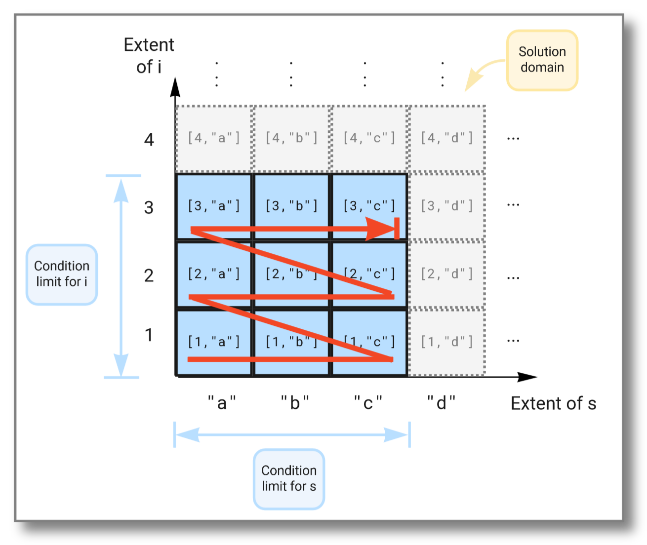
For example, consider the select statement below. It forms a Cartesian product of the extent of i, which is the set of all possible integers, with the extent of s, which is the set of all possible strings. The where clause has two conditions. One that limits i to the set $\{1,2,3\}$, and one that limits s to the set $\{"a","b","c"\}$. This restricts the result to the Cartesian product of $\{1,2,3\}$ and $\{"a","b","c"\}$.

select i, s
  from Integer i, Charstring s
 where i in (values 1,2,3)
   and s in (values "a","b","c");

Running the above query gives the following result:

[1,"a"]
[1,"b"]
[1,"c"]
[2,"a"]
[2,"b"]
[2,"c"]
[3,"a"]
[3,"b"]
[3,"c"]

The figure below illustrates how the extents span the solution domain, and how the result is produced as the Cartesian product of the two extents limited by the conditions in the where clause:

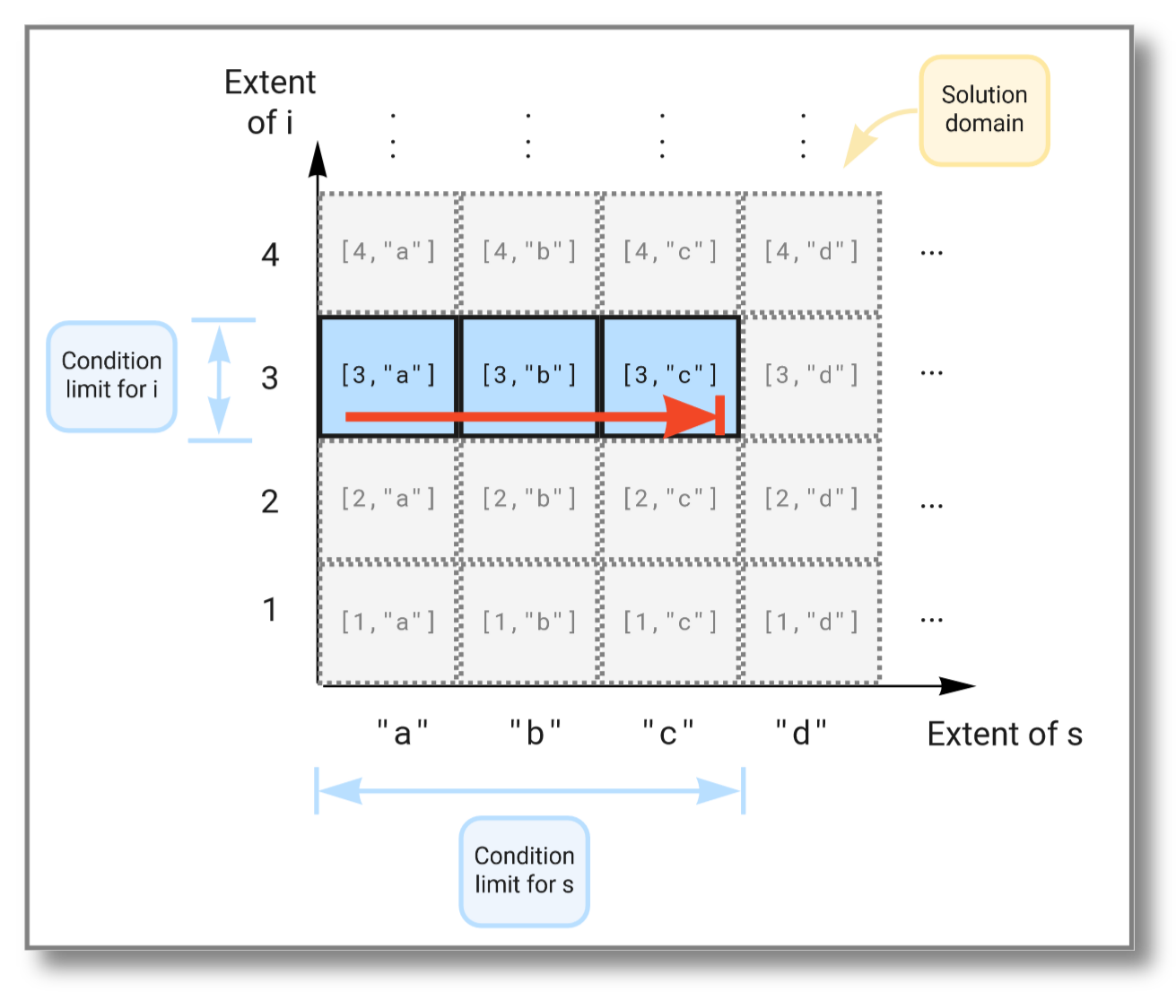
We can limit the solution further by imposing additional conditions in the where clause, like this:

select i, s
  from Integer i, Charstring s
 where i in (values 1,2,3)
   and s in (values "a","b","c")
   and i > 2;

Running the above query gives the following result:

[3,"a"]
[3,"b"]
[3,"c"]

This time the subset of the solution space is further limited due to the extra condition on i and now looks like this:

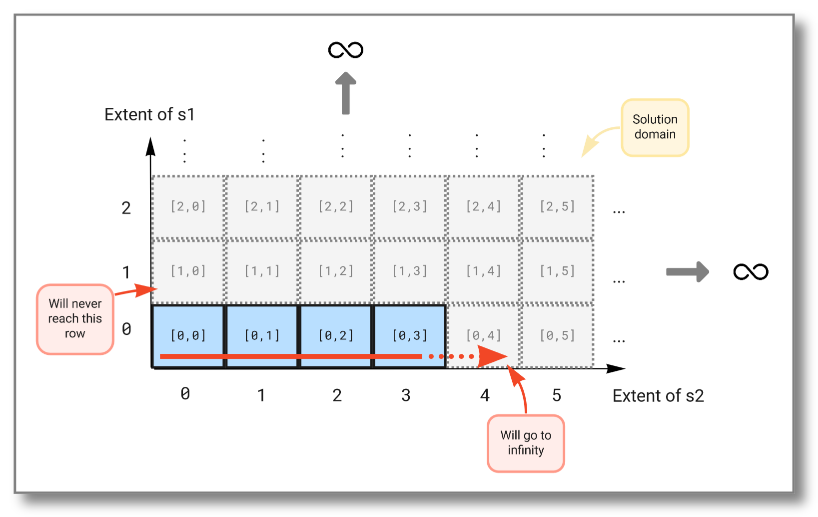
For a stream query, let's consider binding variables to infinite subsets in the solution domain. We can do this by using streams that never end. For example, heartbeat() generates a stream of seconds emitted at a given pace. This stream is infinite since time has no end. The select statement below tries to combine two such streams, but as we will see, taking the Cartesian product between two infinite sets will not work. Try running the query:

select s1, s2
  from Real s1, Real s2
 where s1 in extract(heartbeat(1))
   and s2 in extract(heartbeat(1));

The result should be:

[0,0]
[0,1]
[0,2]
[0,3]
.
.
.

We see that the first stream never increases because the second stream (which is evaluated first) never finishes. The figure below illustrates how the Cartesian product "travels" through the solution domain:

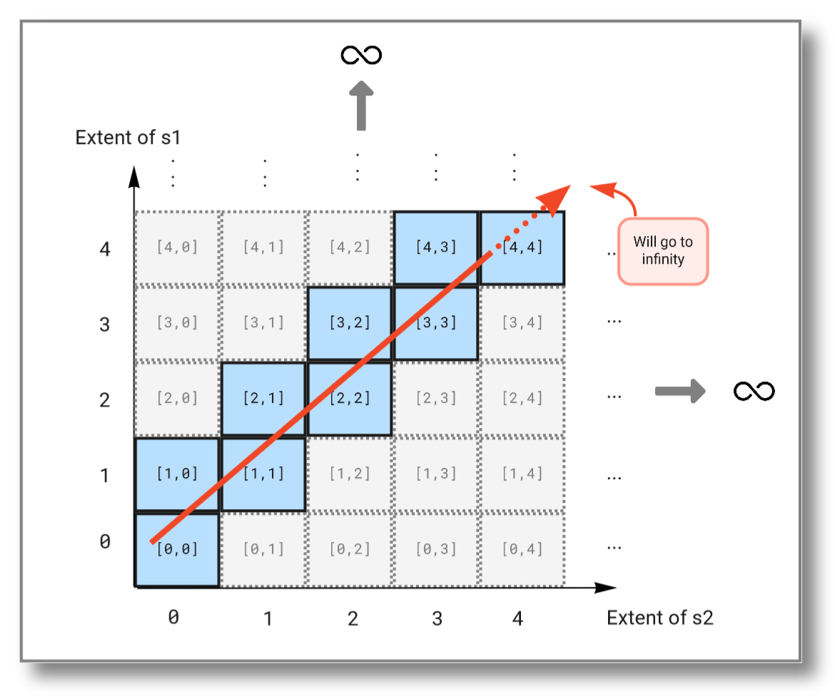
To combine infinite streams you must instead use the pivot() function. It combines the outputs of multiple streams into one vector and outputs a new vector each time one of the streams emits a result. The query below combines the streams from the previous example into a single stream:

select v
  from Stream of Real s1, Stream of Real s2, Vector v
 where s1 = heartbeat(1)
   and s2 = heartbeat(1)
   and v in extract(pivot([s1,s2]));

The result should be:

[0,null]
[0,0]
[1,0]
[1,1]
[2,1]
[2,2]
[3,2]
[3,3]
[4,3]
[4,4]
.
.
.

As you see, this query will continue to infinity but include the values from both streams. If we look at the subset emitted from the solution domain, we see that the query "travels" diagonally through the solution domain:

Visualizing streams

You can use Multi plot for flexible stream visualization.

You can prefix a stream query with a JSON record specifying how to visualize the result. For example, the following query is visualized by a sliding line plot over the latest 200 values:

//plot: Multi plot
{'sa_plot': 'Line plot', 'memory': 200};
select [sin(x), cos(x)]
  from Real x
 where x in extract(10*heartbeat(.02))

Trigonometric functions lend themselves to algebraic manipulation over streams, like this amplitude modulation example:

//plot: Multi plot
{'sa_plot': 'Line plot', 'memory': 200};
select [sin(x)*sin(x/30), cos(x)*cos(x/30)]
  from Real x
 where x in extract(20*heartbeat(.01))

which is more appealing in parametric coordinates (scatter plot):

//plot: Multi plot
{'sa_plot': 'Scatter plot', 'memory': 1000};
select [sin(x)*sin(x/30), cos(x)*cos(x/30)]
  from Real x
 where x in extract(10*heartbeat(.005))

Visualizing reduced streams

Let's assume the following simulated test stream of pairs :sts.

set :sts = (select Stream of [x,y]
              from Real x, Real y
             where x in heartbeat(0.1)
               and y = x * sin(5 * x))

Test :sts:

//plot: Multi plot
{'sa_plot': 'Scatter plot', 'memory': 200};
:sts

Let's make a streamed reducer to scatter plot :sts with different colors depending on whether the y-coordinate in :sts is larger or smaller than the running maximum y-coordinate. For this we need to define a color stream cmax(S) that, for a given stream $S$ with elements $e_i$ returns a stream with elements $f_i = [x_i,y_i,max(y_1...y_i),color(y_i)]$.

Each new $f_i$ is computed from $cmax_{i-1}$ and $e_i$ with this function:

create function cmax_reducer(Vector of Real c, Vector of real e)
                           -> Vector of Real next_c
    as [e[1],                      -- x_i 
        e[2],                      -- y_i 
        max(c[3], e[2]),           -- max(y_1...y_i) 
        case when e[2] > c[3]
             then 0                -- blue
             else 1                -- red
         end]

//plot: Multi plot
{
  "sa_plot": "Scatter plot",
  "size_axis": "none",
  "color_axis": 4,
  "memory": 200
};
reduce(:sts, 'cmax_reducer', [0,0,0,0])

Functions

Basic stream functions are documented in Stream functions.

Functions forming windows over streams are documented in Windowing functions.

Functions to handle named dataflows are documented in Dataflow functions.

Functions to define ontologies over streams are documented in Sensor ontology functions.