Combining streams

In this section we will go through how to combine several streams in a query. This tutorial might help you if you are working with streams of several signals and would like to combine and compare them.

Merging streams

The function merge(Vector of Stream vs)->Stream creates a new stream from the streams in vs. The elements of the merged stream are taken from each of the incomong streams in vs as the arrive.

Example:

timeout(merge([heartbeat(0.25), heartbeat(0.5)*2]),3.1)

The elements of the first stream are 0,0.25,0.5,0.75,1,1.25,1.5,1.75,2,2.25,2.5,2.75,3 produced with pace 0.25 seconds, while the elements of the second stream are 0,1,2,3,4,5,6 produced with pace 0.5 second.

The merge() function is used when the same elements are retrieved from different sources and there is no need to identify the origin of each element.

Pivot streams

The function pivot(Vector of Stream vs)->Stream of Vector merges a vector of streams $VS$ into a pivoted stream of vectors $PS$ where each element $PS_i$ is the most recently received value from some stream $VS_i$ in $VS$.

Example: The following query merges two different heartbeat streams:

select pivot([heartbeat(0.5), heartbeat(1)])
 limit 10

info

Notice that the first vector contains a null value. This is because the pivoted stream had not received any value from the second stream when it received the first value from stream 1. This can be avoided by using a pivot streams variant that takes an extra argument being the initial vector in the result stream:

pivot([heartbeat(0.5), heartbeat(1)], [0,0])

The following query returns a stream of the currently largest elements in the incoming streams:

select max(pivot([sin(heartbeat(0.25)), sin(heartbeat(0.5))]))
 limit 15

Unlike merge(), pivot() makes it possible to identify the origin of each element of the result stream by accessing elements of each pivoted result stream element.

Example: The following query returns a stream where each element contains both the index of the incoming stream producing the maximum value and the value itself:

select argmax(m), max(m)
  from Vector of Real m
 where m in pivot([sin(heartbeat(0.25)), sin(heartbeat(0.5))])
 limit 15

Let's time stamp the elements:

select ts([argmax(m), max(m)])
  from Vector of Real m
 where m in pivot([sin(heartbeat(0.25)), sin(heartbeat(0.5))])

info

When time stamping query result tuples that have several values they must be placed in vectors.

Now let's pivot two simulated streams:

select v
  from Stream of Vector pivot, Vector of Stream vs, Vector v
 where vs = [1+simstream(0.02), 2+simstream(.2)]
   and pivot = pivot(vs)
   and v in pivot
 limit 14

select v
  from Stream of Vector pivot, Vector of Stream vs, Vector v
 where vs = [1+simstream(0.02), 2+simstream(.2)]
   and pivot = pivot(vs, zeros(dim(vs)))
   and v in pivot
 limit 14

The following is an example of a more advanced stream pivot:

select pivot
  from Stream of Vector pivot,
       Vector of Stream vs,
       Stream heartbeat_mod,
       Stream fast_heartbeat_mod
 where vs = [
              simstream(0.02),
              3+simstream(.2),
              heartbeat_mod,
              fast_heartbeat_mod
            ]
   and heartbeat_mod = 1 - 2*mod(heartbeat(1), 2)
   and fast_heartbeat_mod = mod(round(10*heartbeat(.1)), 2)
   and pivot = pivot(vs, zeros(dim(vs)))
 limit 14

Arithmetics on combined streams

If you want to run arithmetics on pivoted streams you first need to extract the vectors from the pivoted stream. This is done with the line v in sv in the query below.

//plot: Line plot
select v[1]*v[4] + v[3]*10, v[4], v[2]
  from Stream of Vector sv,
       Vector of Stream vs,
       Stream hbmod,
       Stream hbmodfast,
       Vector of Real v
 where hbmod = 1 - 2*mod(heartbeat(1), 2)
   and hbmodfast = mod(round(10*heartbeat(.1)), 2)
   and vs = [simstream(0.02), 3+3*simstream(.2), hbmod, hbmodfast]
   and sv = pivot(vs, zeros(dim(vs)))
   and v in sv
 limit 100

Let's smooth that v[2]

//plot: Line plot
select v[1]*v[4] + v[3]*10, v[4], avg(win)
  from Stream of Vector sv,
       Vector of Stream vs,
       Stream hbmod,
       Stream hbmodfast,
       Vector of Real v,
       Vector of Real win
 where hbmod = 1 - 2*mod(heartbeat(1), 2)
   and hbmodfast = mod(round(10*heartbeat(.1)), 2)
   and vs = [simstream(0.02), winagg(3+3*simstream(.2),10,1),
             hbmod, hbmodfast]
   and sv = pivot(vs, zeros(dim(vs)))
   and v in sv
   and win = v[2]
 limit 100

The following two queries seem to be defined in the same way, but they do give rise to different behavior:

//plot: Multi plot
{'sa_plot': 'Scatter plot', 'labels':['x','y'], 'memory': 1000};
select pivot([sin(10*heartbeat(.01)),
              cos(10*heartbeat(.01))])
 limit 150

//plot: Multi plot
{'sa_plot': 'Scatter plot', 'labels':['x','y'], 'memory': 1000};
select sin(x), cos(x)
  from Real x
 where x in 10*heartbeat(.02)
 limit 50

Note

The first query differs slightly since it uses two independent streams together with pivot streams, This means that we essentially have two streams where sin and cos are applied to their own stream over time (heartbeat) before they are merged.

In the second example we apply sin and cos to the x from the same heartbeat stream.

More examples of how we can specify multiple streams in a query:

//plot: Multi plot
{'sa_plot': 'Line plot', 'memory': 200};
select pivot([sin(hb), sin(hb+pi())])
  from Stream of Real hb
 where hb = 10*heartbeat(.02)
 limit 100

//plot: Multi plot
{'sa_plot': 'Bar plot', 'memory': 200};
select pivot(select Vector of sin(i/3 + 3*heartbeat(.03))
               from Integer i
              where i in range(0,29)
              order by i)
 limit 100

Hopefully these short examples have made you understand how you can combine streams.

Type extents and the solution domain

We explain the theory behind how select stream queries combine infinite sets of objects and show how this is used for combining infinite streams.

Every type t has an extent(t) being the set of all objects of type t. For example, the extent of the type Integer is "all integers from negative infinity to positive infinity", or $\{-\infty, ..., -2, -1, 0, 1, 2, ..., \infty\}$.

A select statement first forms the Cartesian product of the extents of all variables in the from clause, called the solution domain. The where clause then specifies conditions limiting the emitted result to a subset of the solution domain.

For example, consider the select statement below. It forms a Cartesian product of the extent of i, which is the set of all possible integers, with the extent of s, which is the set of all possible strings. The where clause has two conditions. One that limits i to the set $\{1,2,3\}$, and one that limits s to the set $\{"a","b","c"\}$. This restricts the result to the Cartesian product of $\{1,2,3\}$ and $\{"a","b","c"\}$.

select i, s
  from Integer i, Charstring s
 where i in bag(1,2,3)
   and s in bag("a","b","c");

Running the above query gives the following result:

[1,"a"]
[1,"b"]
[1,"c"]
[2,"a"]
[2,"b"]
[2,"c"]
[3,"a"]
[3,"b"]
[3,"c"]

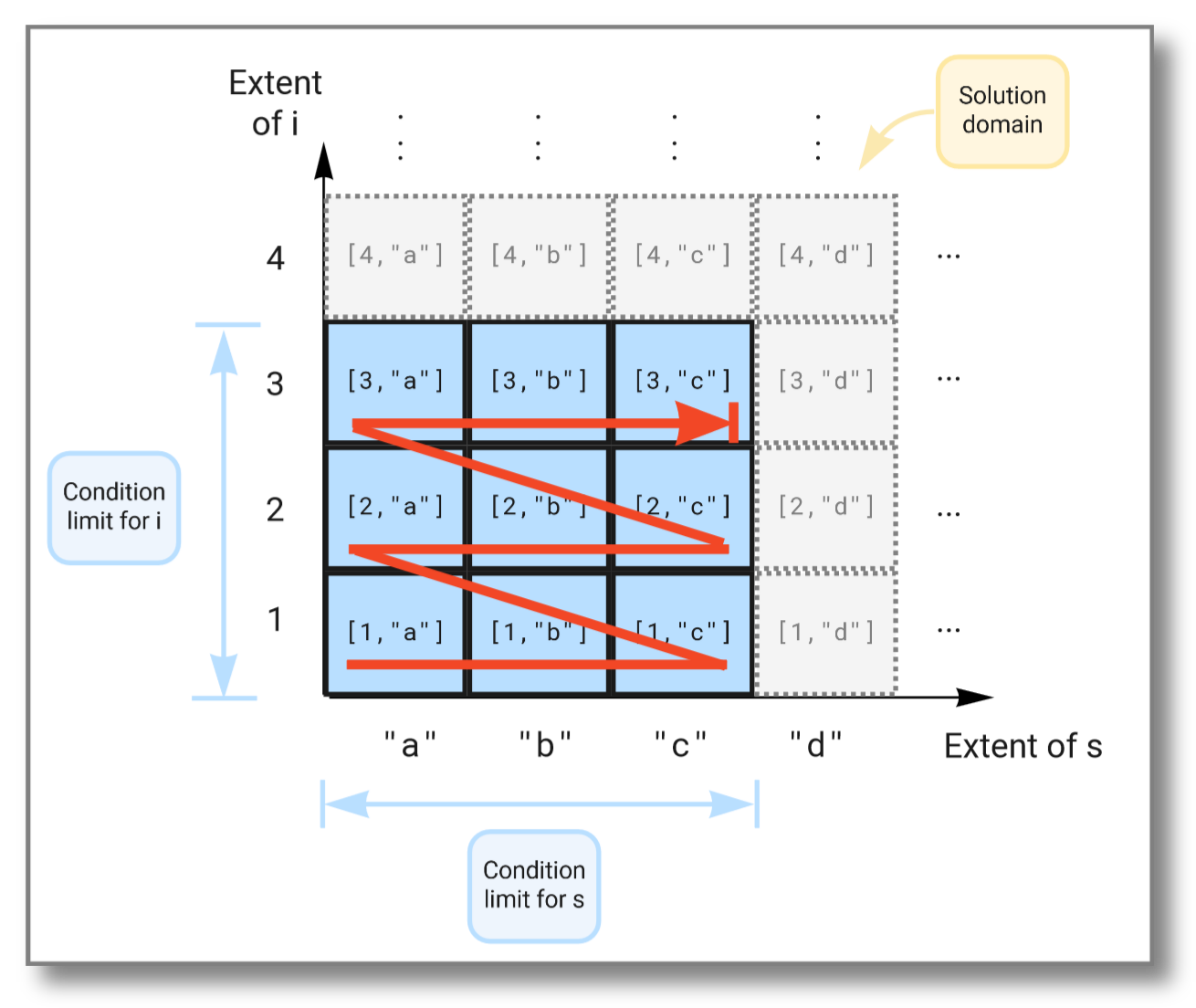
The figure below illustrates how the extents span the solution domain, and how the result is produced as the Cartesian product of the two extents limited by the conditions in the where clause:

We can limit the solution further by imposing additional conditions in the where clause, like this:

select i, s
  from Integer i, Charstring s
 where i in bag(1,2,3)
   and s in bag("a","b","c")
   and i > 2;

Running the above query gives the following result:

[3,"a"]
[3,"b"]
[3,"c"]

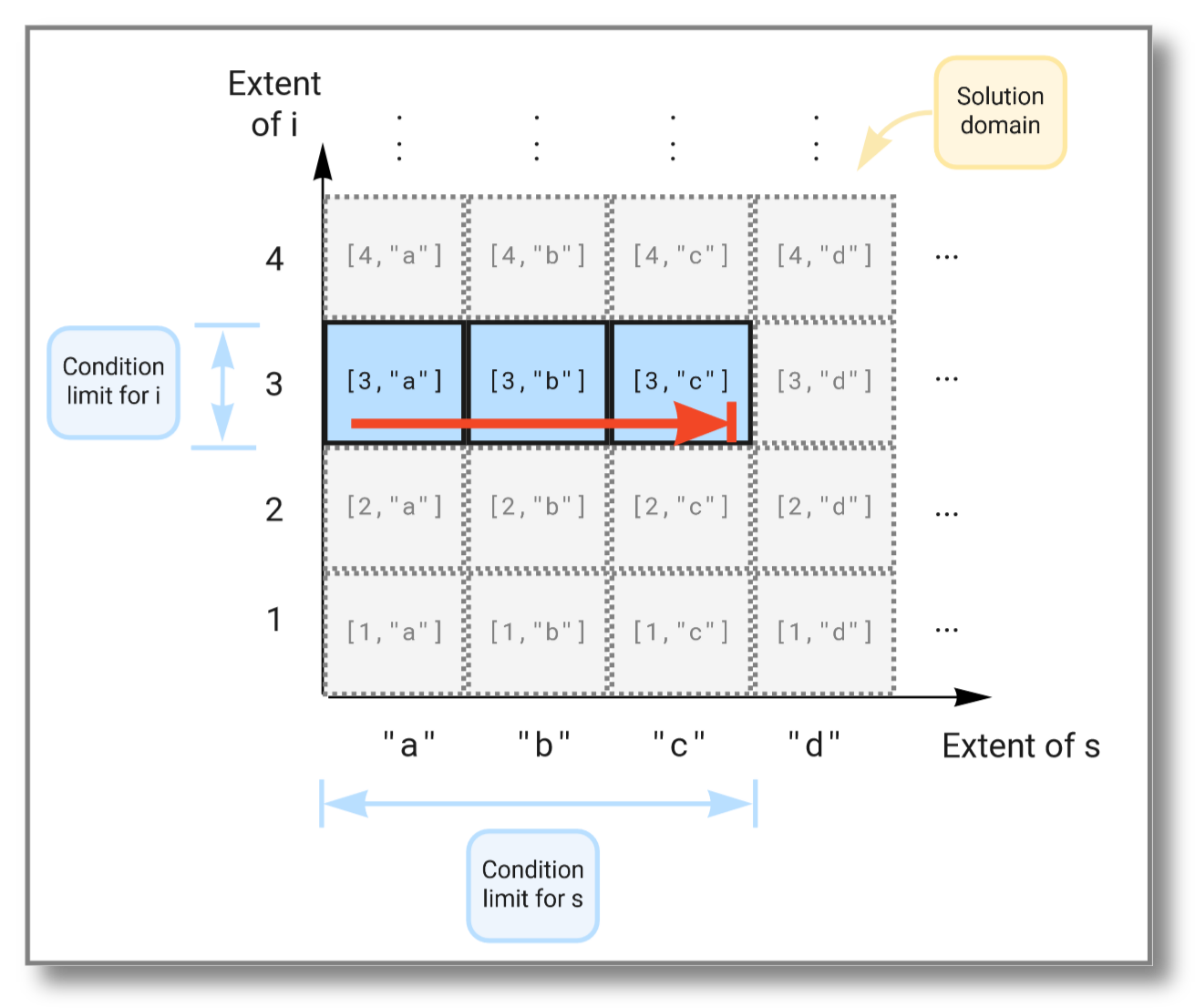
This time the subset of the solution space is further limited due to the extra condition on i and now looks like this:

For a stream query, let's consider binding variables to infinite subsets in the solution domain. We can do this by using streams that never end. For example, heartbeat() generates a stream of seconds emitted at a given pace. This stream is infinite since time has no end. The select statement below tries to combine two such streams, but as we will see, taking the Cartesian product between two infinite sets will not work. Try running the query:

select s1, s2
  from Real s1, Real s2
 where s1 in heartbeat(1)
   and s2 in heartbeat(1);

The result should be:

[0,0]
[0,1]
[0,2]
[0,3]
.
.
.

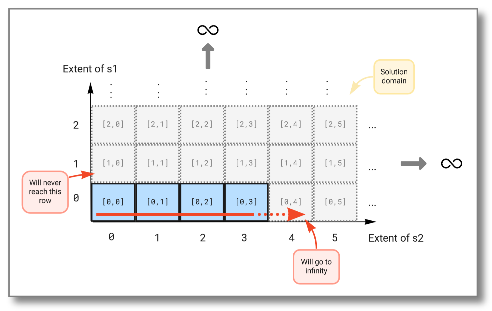
We see that the first stream never increases because the second stream (which is evaluated first) never finishes. The figure below illustrates how the Cartesian product "travels" through the solution domain:

To combine infinite streams you must instead use the pivot() function. It combines the outputs of multiple streams into one vector and outputs a new vector each time one of the streams emits a result. The query below combines the streams from the previous example into a single stream:

select v
  from Stream of Real s1, Stream of Real s2, Vector v
 where s1 = heartbeat(1)
   and s2 = heartbeat(1)
   and v in pivot([s1,s2]);

The result should be:

[0,null]
[0,0]
[1,0]
[1,1]
[2,1]
[2,2]
[3,2]
[3,3]
[4,3]
[4,4]
.
.
.

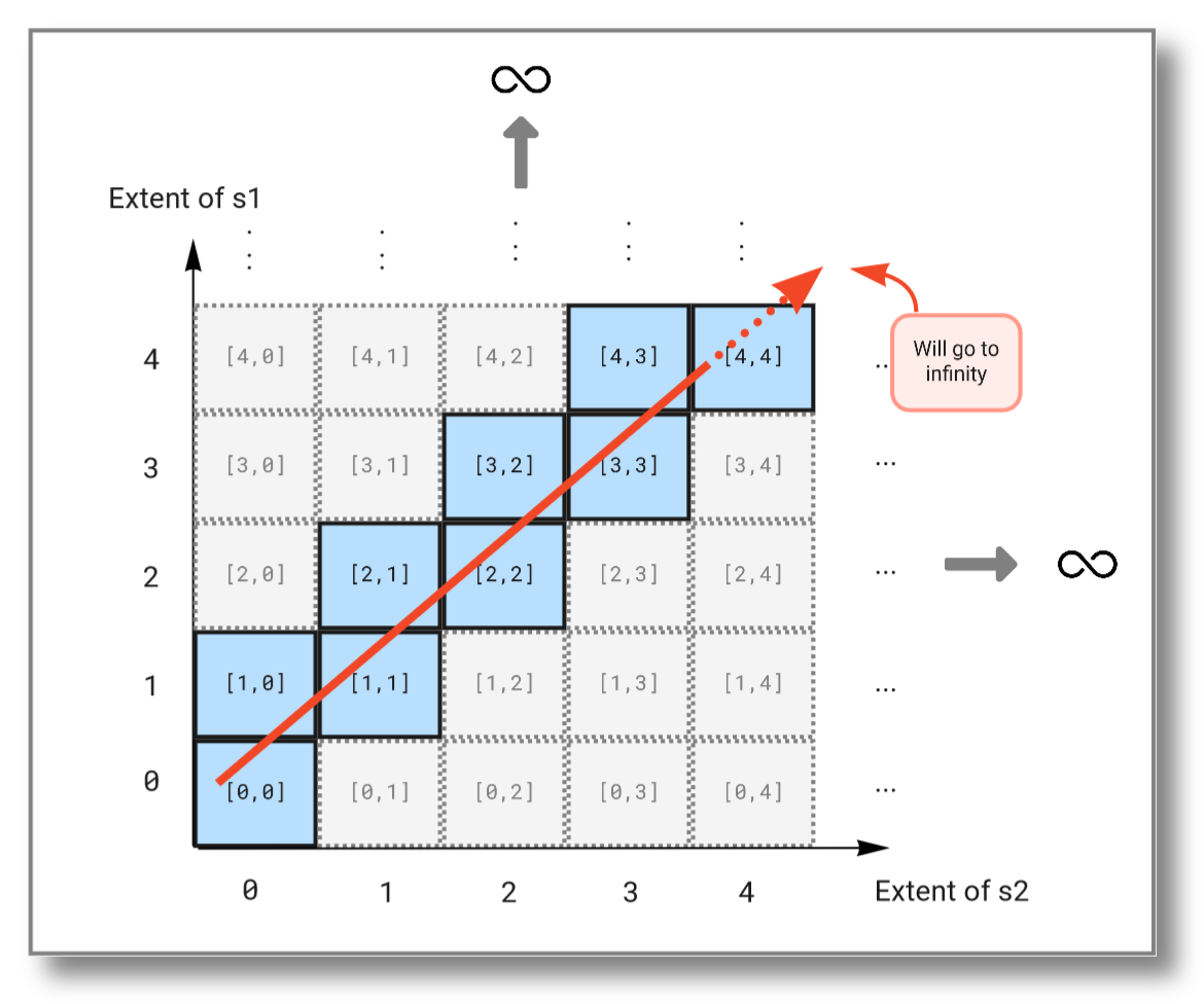
As you see, this query will continue to infinity but include the values from both streams. If we look at the subset emitted from the solution domain, we see that the query "travels" diagonally through the solution domain:

select i
  from Integer i, Vector v
 where v = [4,3,9,1,9,5]
   and v[i] = max(v);