Streams

A stream is a possibly infinite sequence of elements. It often grows over time at some pace.

Example: The following query returns an infinite stream of the elapsed time every 0.5 seconds.

heartbeat(0.5)

Note

The query is an example of a continuous query (CQ) since it continuously produces objects. You can explicitly stop it pressing the stop_circle button.

You can apply computational functions on streams. The applied function will then be applied on each element of the stream.

Example:

sqrt(heartbeat(0.5))

The select Stream of syntax provides a very flexible way of defining new streams out of other ones. This is called a select stream query.

Example:

select Stream of x
  from Real x
 where x in extract(heartbeat(0.5))
   and mod(x,1) < 0.1

Note

The syntax e in extract(s) extracts elements e from the stream s so they can be used in select queries.

Visit Select stream queries for more on select stream queries.

You can stop an infinite CQ after a specific number of elements by specifying a limit in a select query.

Example:

select heartbeat(0.125)
 limit 5

You can also stop a CQ after a specific number of seconds by using the timeout(s,limit) function.

Example:

timeout(heartbeat(0.125),0.9)

You can assign a stream to a variable without running it.

Example:

set :s = heartbeat(0.5)

This runs the stream object bound to session variable :s:

:s

You can create tuple streams whose elements are several values paired together as tuples.

Example:

select Stream of hb, sin(hb)
  from Number hb
 where hb in heartbeat(0.5)
   and sin(hb) > 0.1

You can label stream elements by adding identifiers in stream tuples.

Example:

set :s1 = (select Stream of 's1', hb
             from Number hb
            where hb in heartbeat(0.5))

:s1

You can combine streams using system functions taking more than one stream as argument.

Example: the function merge(Stream s1,Stream s2)->Stream combines the elements of two streams as they arrive producing a merged stream:

merge(heartbeat(0.5), heartbeat(0.6))

Labeled tuple streams can be combined with merge.

Example: Let's create another labeled stream :s2.

set :s2 = (select Stream of 's2', hb
             from Number hb
            where hb in heartbeat(0.6))

Combine :s1 and :s2:

merge(:s1, :s2)

The result from the merge produces a bus stream of labels, called signals and the corresponding values.

You can convert a bus stream for a given vector of labels keys into a stream of vectors of corresponding values by calling pivot_bus(Vector keys,Stream bus)->Stream of Vector.

Example:

pivot_bus(['s1','s2'],merge(:s1, :s2))

Visit Combining streams for more on how to combine data streams.

Visualizing streams

The result can be visualized in real time.

Example:

//plot: line plot
sin(10*heartbeat(0.01)) 

You can produce 2D coordinate vectors [x,y] from the stream and plot them as 2D-points in a scatter plot.

Example:

//plot: Scatter plot
select Stream of [x,y]
  from Real x, Real y
 where x in heartbeat(0.1)
   and y = x * sin(5*x)

You can make your own simulated sine stream function of coordinates.

Example:

create function my_stream() -> Stream of Vector of Real
  as select Stream of [x,y]
       from Real x, Real y
      where x in heartbeat(0.1)
        and y = x * sin(5*x)

//plot: Scatter plot
my_stream()

We can also make a colored scatter plots of my_stream.

//plot: Multi plot
{
  "sa_plot": "Scatter plot",
  "color_axis": 2        -- Plot each different Y with different color
};
my_stream()

Visit Stream visualization for more on stream visualization.

Stream windows

Windows forming functions continuously construct windows over a stream. The windows are represented as vectors, so the window forming functions convert an input stream of elements to a stream of vectors of elements. The function winagg() is a count-based window function and the function twinagg() is a time-based window function, as explained next.

Count windows

The window forming function winagg(Stream s,Number size,Number stride)->Stream of Vector creates a count-based stream of windows from an input stream s. You specify the number of stream elements that each window contains (the window size) and how many stream elements the window moves forward before emitting the next window (the stride).

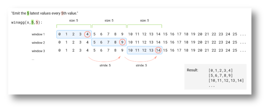
To create a tumbling window (a non-overlapping window) you provide the same value for size and stride.

Example: The following query produces a tumbling window.

winagg(heartbeat(1), 5, 5)

Since heartbeat(1) generates a stream element per second, it takes 5s for the query to output the first result. You can read the query as "emit the 5 latest elements every 5th element". The figure below illustrates the behavior of this query:

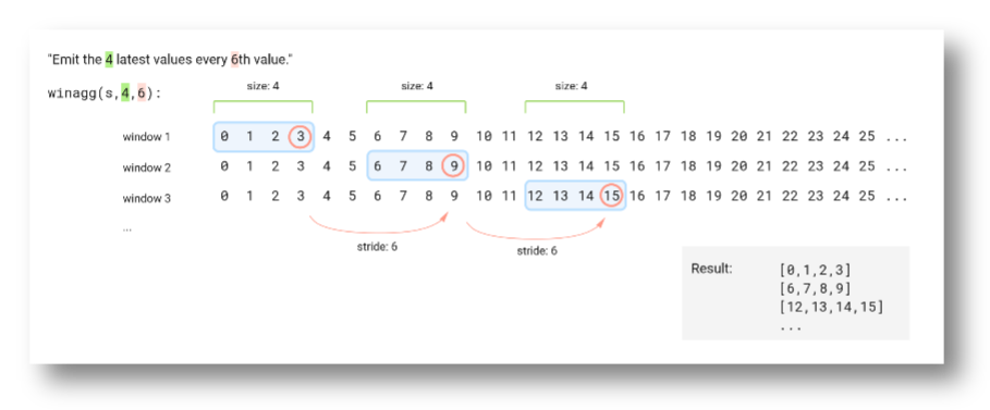
It is not required to keep all the elements in the input stream. You can specify a stride that is larger than the window size. Doing this will sample the stream every stride element.

Example:

winagg(heartbeat(1), 4, 6)

You can read the query as "emit the 4 latest elements every 6th element". It effectively skips two elements between every window, which is illustrated in the figure below:

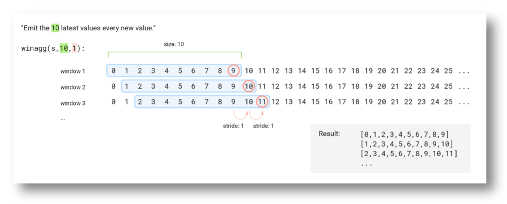
You get sliding windows having overlapping elements by specifying a stride value that is lower than the window size.

Example:

winagg(heartbeat(1), 10, 1)

The query produces a 10-element window every time the input stream emits a new element, which is illustrated in the figure below:

Temporal windows

The window forming function twinagg() is a time-based window function that creates a stream of temporal windows from an input stream of time stamped objects. It works much like winagg() but instead of specifying window size and stride in number of elements you specify it in seconds.

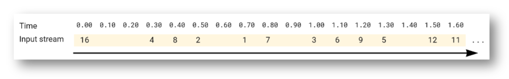
We will use a custom stream to illustrate how twinagg() works. We assign the variable :s1 to a finite stream of explicit time stamped objects.

set :s1 = stream ts(|2022-05-12T00:00:00.0Z|,16),
                 ts(|2022-05-12T00:00:00.3Z|,4),
                 ts(|2022-05-12T00:00:00.4Z|,8),
                 ts(|2022-05-12T00:00:00.5Z|,2),
                 ts(|2022-05-12T00:00:00.7Z|,1),
                 ts(|2022-05-12T00:00:00.8Z|,7),
                 ts(|2022-05-12T00:00:01.0Z|,3),
                 ts(|2022-05-12T00:00:01.1Z|,6),
                 ts(|2022-05-12T00:00:01.2Z|,9),
                 ts(|2022-05-12T00:00:01.3Z|,5),
                 ts(|2022-05-12T00:00:01.5Z|,12),
                 ts(|2022-05-12T00:00:01.6Z|,11)

If we illustrate the time stamped stream :s1 on a timeline it looks like this:

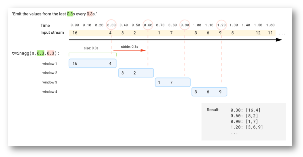
To create a non-overlapping time window (a tumbling window) you provide the same value for size and stride. Try it by running the following query:

twinagg(:s1, 0.3, 0.3)

The figure below illustrates how the tumbling window passes over the stream elements:

Just like with winagg(), twinagg() can also skip elements by specifying a stride that is larger than the window size, or use a sliding window by specifying a stride that is smaller than the window size.

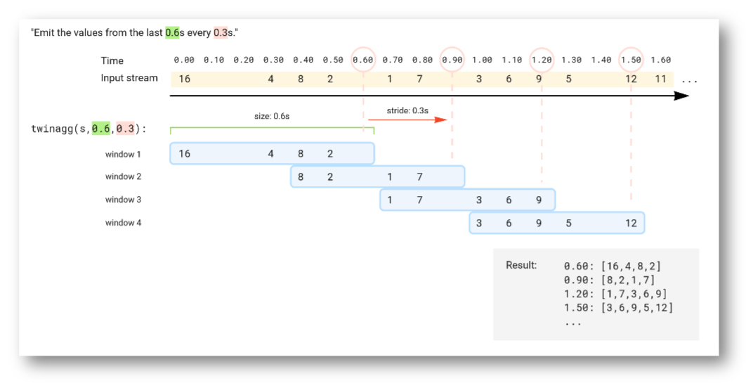
Here is an example where window size is larger than the stride. Try it by running the query:

twinagg(:s1, 0.6, 0.3)

The query produces a 0.6 second window every 0.3 seconds, which is illustrated in the figure below:

Streamed aggregation

Regular aggregate functions such as sum and count cannot be called for steams. The reason is streams are continuously growing and potentially infinite. Instead, there are special running aggregate functions for streams that for a given stream $S$ with elements $e_i$ returns a stream of aggregated values of elements $e_1,...,e_i$.

The built-in running aggregation function rsum(Stream of Number s)->Stream of Number computes the running sum of the stream s, while rcount(Stream s)->Stream of Integer computes the running count.

Examples:

rsum(diota(0.5,1,5))

rcount(diota(0.5,1,5))

Streamed reduce

Often one would like to make customized aggregations over streams. For this, one can use streamed reduce using the reduce function. It behaves differently for streams than for other collections. When reduce is applied on a stream s it will produce a stream of running aggregated values for each element in s using one pass reduction. Often the same one-pass reducer as for bags can be used.

Example: The following query returns the running maximum of the stream sin(diota(0.25,1,9)).

reduce(sin(diota(0.25,1,9)),'max')

Unlike reduce over other collections, streamed reduce allows the collection of both running aggregated values along with individual stream elements, since with streamed reduce a new result is returned for every element in the stream.

Example: Let's define a stream $R$ of running maximum values pairs of a stream $S$. If$S$ has the elements $e_i = [x_n,y_n]$, the stream $R$ will have the elements $emax_i = [x_i,max(y_1,...,y_i)]$.

The recurrence formulas are as follows.

Initialization: $\newline emax_1 = e_1 \newline$ Reduction: $\newline emax_i = [x_{i,1}, max(emax_{i-1,2},x_{i,2})] \newline$

Based of the recurrence formulas we define the reducer as follows.

create function emax_reducer(Vector emax, Vector e)
                           -> Vector next_emax
  as [e[1],
      max(emax[2], e[2])]

Now we can use simple streamed reduce to define emax.

create function emax(Stream of Vector s) -> Stream of Vector
  as reduce(s, 'emax_reducer')

Test it:

emax(stream [1,1],[2,4],[3,2],[4,6])

For more examples of streamed reduce, visit Streamed reduce.

Visit the reference section Streams for more on queries and functions over streams.