Queries over infinite streams

🚀 Interactive documentation

This page uses Wasm code blocks so you can run the examples directly in the browser.

One important feature of the OSQL language is to enable processing functions and filters over streams. A stream is a possibly infinite sequence of objects. It often grows continuously over time at some pace.

Continuous queries

The function heartbeat(pace) returns a stream of numbers representing the time elapsed from its start every pace seconds.

Example:

heartbeat(0.5)

Note

The query is an example of a continuous query (CQ) since it continuously produces an infinite stream of results until you explicitly stop it by pressing the stop button.

The following CQ returns a continuous sine wave if visualized as a line plot:

//plot: Line plot
select sin(10*x)
  from Number x
 where x in heartbeat(0.05)

The same query can also be expressed as:

//plot: Line plot
sin(10*heartbeat(0.05))

Note

heartbeat is a stream generator, i.e. a function that returns a stream as an object. The in operator extracts the elements from a stream. If a simple function like sin or operator like * is applied on a stream generator it will be applied on each element of the stream thus generating a transformed stream as in the example.

You can stop an infinite CQ by specifying a limit in a select query, for example:

select sin(10*heartbeat(0.05)) limit 5

The query optimizer also allows applying functions on entire streams, for example:

//plot: Line plot
select sin(s)
  from Stream of Number s
 where s=10*heartbeat(.01)

can also be expressed as:

//plot: Line plot
sin(10*heartbeat(.01))

Synthetic streams

The built-in library of trigonometric functions is very useful for generating synthetic streams. For example, the function simstream(Number pace) returns a simulated stream of numbers with given pace.

Example:

//plot: Line plot
simstream(0.1)

It is defined as simsig(heartbeat(pace)), thus calling the function simsig(x) each x seconds after its start at the given pace. This is an example of how to generate a synthetic stream.

Exercise

Inspect the definitions of simstream() and simsig() to see how they are defined.

The function ts_simstream(pace) produces a stream of numbers where each element is time stamped with the wall time when it was produced. This is called a , a time stamped stream.

Example:

//plot: Line plot
ts_simstream(0.01)

info

Notice that the X-labels indicate the times when each element was produced. If you wait a while you will see how the stream start scrolling to the left.

Time stamped streams can be defined by adding time stamps to the elements x of a stream's result by calling the function ts(x). For example, the following query returns the same timestamped simulated stream of numbers as ts_simstream(0.01):

//plot: Line plot
select Stream of ts(x)
  from Number x
 where x in simstream(0.01)

The function ts(x) returns a time stamped object having the value x (see Time).

Exercise

Visualize the four first elements of the time stamped stream as text.

The function sample_stream(x, pace) returns an infinite stream of the expression x evaluated every pace seconds, for example:

sample_stream("Hello stream",1)

The following CQ returns a visualized stream of time stamped random numbers:

//plot: Line plot
sample_stream(ts(rand(100)),0.1)

Stream filters

CQs can be defined that filter out stream elements fulfilling user defined conditions using a select Stream of query. For example, the following CQ filters out the stream elements of simstream(0.1) larger than 0.7 visualized as a line plot:

//plot: Line plot
select Stream of x
  from Number x
 where x in simstream(0.01)
   and x > 0.7

The CQ generates a new stream of the selected stream elements. Notice how the result stream pauses (slows down) when when elements less than 0.7 are produced by simstream(0.01).

Stream windows

The CQ examples we have seen so far generate infinite streams of single values (strings or numbers). However, it is often necessary to operate on streams of finite sections of the latest elements of a stream, called stream windows, e.g. a stream of the latest 10 elements in an infinite stream. In OSQL windows are represented as vectors. There are several built-in functions in sa.engine for forming such streams of windows.

Forming windows with winagg

Try this CQ visualized as Bar plot:

//plot: Bar plot
winagg(sin(heartbeat(0.1)*5),10,10)

It produces a stream of vectors (i.e. windows) by collecting into the vectors 10 elements at the time from the stream sin(heartbeat(0.1)*5).

Exercise

Visualize the four first elements of the stream as text.

Since heartbeat(0.1) produces a number 10 times per second and the windows contain 10 elements, the result from the expression is a stream of vectors produced once per second, i.e. with pace 1 HZ.

Tumbling and sliding windows

In general the function winagg(s, size, stride) forms a stream of windows of given size over a stream s. The third parameter stride defines the how many stream elements the window moves forward over the stream, called its stride. In our example above the size and the stride are both 10, meaning that once a window of 10 elements is produced a new one is started to be formed. This is called a tumbling window.

If the stride is smaller than the size, new overlapping windows will be produced more often. This is called a sliding window.

Example:

//plot: Bar plot
winagg(sin(heartbeat(0.1)*5),10,2)

Moving average

A common way to reduce noisy signals is to form the moving average of sliding windows over a stream of measurements by computing the average mean(w) for each window w.

Example:

//plot: Line plot
mean(winagg(simstream(0.01),10,5))

As an alternative, try using median() instead of mean().

Often CQs are defined over windows of elements. For example, this CQ returns the moving averages larger than 0.7 of windows of simstream(0.1):

//plot: Line plot
select Stream of x
  from Number x
 where x in mean(winagg(simstream(0.01),5,5))
   and x > 0.7

Here you will notice rather long pauses.

Temporal windows

The following query produces a stream of time stamped sliding windows each having 10 elements with 50% overlap.

ts(winagg(simstream(0.01),10,5))

Exercise

Visualize the three first elements of the time stamped stream as line plot, bar plot, and text.

The kind of windows discussed so far are called counting windows in that they produce window vectors based on counting the incoming stream elements. This is a very efficient and simple method to form windows, e.g. for continuously computing statistics over windows of arriving data, as the moving average above. It works particular well if the elements arrive at a constant pace.

However, if the elements arrive irregularly one may need to form temporal windows whose sizes are based on elements arriving during a time period rather than on the number of arriving elements. Temporal windows are formed with the OSQL function twinagg(ts, size, Stride) that takes a timestamped stream of objects as input and produces a time stamped stream of vectors of objects as result. The parameters size and 'stride' are here measured in seconds rather than number of elements as winagg().

For example:

select tv
  from Timeval of Vector of Number tv
 where tv in twinagg(ts_simstream(0.01),0.5,0.5)

The following query computes the mean and median of simstream with pace 100HZ each 1/2 second:

//plot: Line plot
select mean(v), median(v)
  from Timeval of Vector of Number tv, Vector of Number v
 where tv in twinagg(ts_simstream(0.01),0.5,0.5)
   and v = value(tv)

Notice that you can apply any Vector function on v.

For more on windows over stream sea Windowing.

The next part of the tutorial shows how to make queries over many streams.

Visualizing streams

We show how to use Multi plot for flexible stream visualization.

You can prefix a stream query with a JSON record specifying how to visualize the result. For example, the following query is visualized by a sliding line plot over the latest 200 values:

//plot: Multi plot
{'sa_plot': 'Line plot', 'memory': 200};
select [sin(x), cos(x)]
  from Number x
 where x in 10*heartbeat(.02)

Trigonometric functions lend themselves to algebraic manipulation over streams, like this amplitude modulation example:

//plot: Multi plot
{'sa_plot': 'Line plot', 'memory': 200};
select [sin(x)*sin(x/30), cos(x)*cos(x/30)]
  from Number x
 where x in 20*heartbeat(.01)

which is more appealing in parametric coordinates (scatter plot):

//plot: Multi plot
{'sa_plot': 'Scatter plot', 'memory': 1000};
select [sin(x)*sin(x/30), cos(x)*cos(x/30)]
  from Number x
 where x in 10*heartbeat(.005)

Type extent and the solution domain

Every type t has an extent(t) being the set of all objects of type t. For example, the extent of the type Integer is "all integers from negative infinity to positive infinity", or $\{-\infty, ..., -2, -1, 0, 1, 2, ..., \infty\}$.

A select statement first forms the Cartesian product of the extents of all variables in the from clause, called the solution domain. The where clause then specifies conditions limiting the emitted result to a subset of the solution domain.

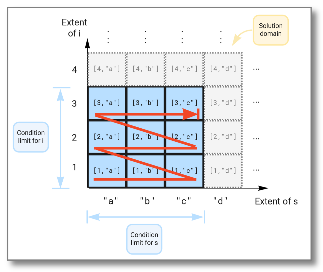
For example, consider the select statement below. It forms a Cartesian product of the extent of i, which is the set of all possible integers, with the extent of s, which is the set of all possible strings. The where clause has two conditions. One that limits i to the set $\{1,2,3\}$, and one that limits s to the set $\{"a","b","c"\}$. This restricts the result to the Cartesian product of $\{1,2,3\}$ and $\{"a","b","c"\}$.

select i, s
  from Integer i, Charstring s
 where i in bag(1,2,3)
   and s in bag("a","b","c");

Running the above query gives the following result:

[1,"a"]
[1,"b"]
[1,"c"]
[2,"a"]
[2,"b"]
[2,"c"]
[3,"a"]
[3,"b"]
[3,"c"]

The figure below illustrates how the extents span the solution domain, and how the result is produced as the Cartesian product of the two extents limited by the conditions in the where clause:

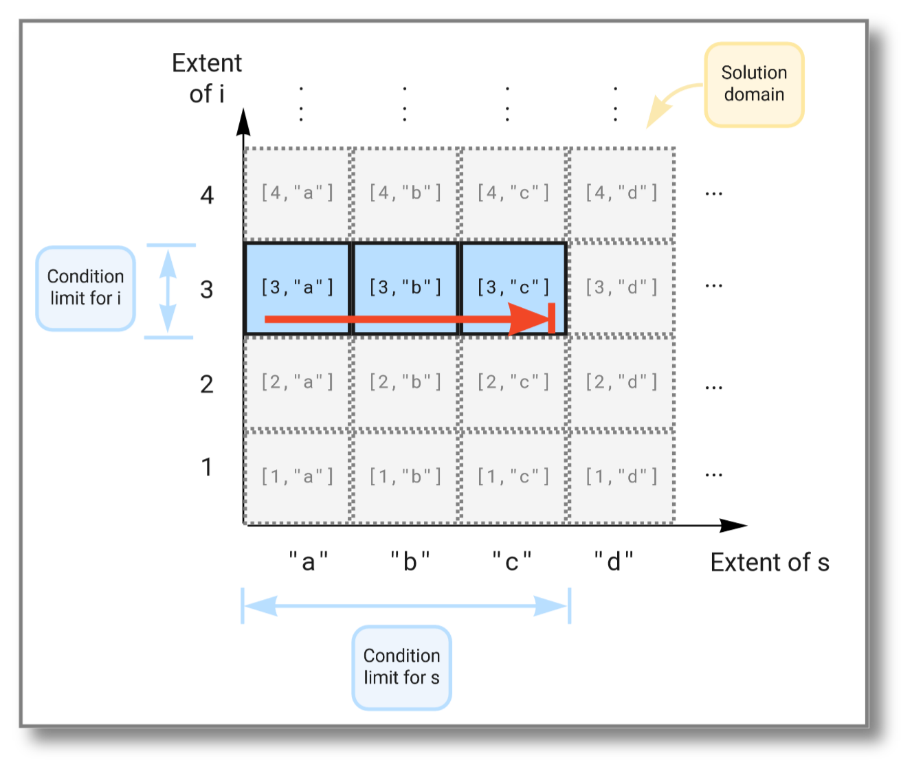
We can limit the solution further by imposing additional conditions in the where clause, like this:

select i, s
  from Integer i, Charstring s
 where i in bag(1,2,3)
   and s in bag("a","b","c")
   and i > 2;

Running the above query gives the following result:

[3,"a"]
[3,"b"]
[3,"c"]

This time the subset of the solution space is further limited due to the extra condition on i and now looks like this:

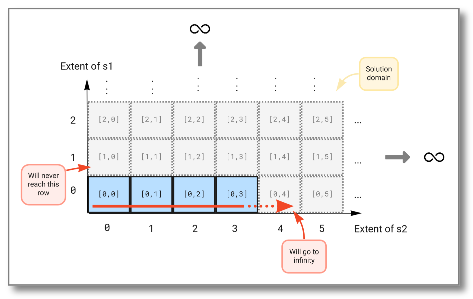
For a Stream query, let's consider binding variables to infinite subsets in the solution domain. We can do this by using streams that never end. For example, heartbeat() generates a stream of seconds emitted at a given pace. This stream is infinite since time has no end. The select statement below tries to combine two such streams, but as we will see, taking the Cartesian product between two infinite sets will not work. Try running the query:

select s1, s2
  from Number s1, Number s2
 where s1 in heartbeat(1)
   and s2 in heartbeat(1);

The result should be:

[0,0]
[0,1]
[0,2]
[0,3]
.
.
.

We see that the first stream never increases because the second stream (which is evaluated first) never finishes. The figure below illustrates how the Cartesian product "travels" through the solution domain:

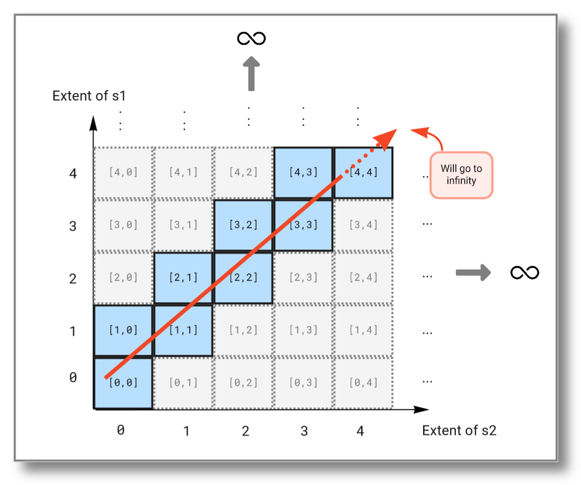
To combine infinite streams you must instead use the pivot() function. It combines the outputs of multiple streams into one vector and outputs a new vector each time one of the streams emits a result. The query below combines the streams from the previous example into a single stream:

select v
  from Stream of Number s1, Stream of Number s2, Vector v
 where s1 = heartbeat(1)
   and s2 = heartbeat(1)
   and v in pivot([s1,s2]);

The result should be:

[0,null]
[0,0]
[1,0]
[1,1]
[2,1]
[2,2]
[3,2]
[3,3]
[4,3]
[4,4]
.
.
.

As you see, this query will continue to infinity but include the values from both streams. If we look at the subset emitted from the solution domain, we see that the query "travels" diagonally through the solution domain:

select i
  from Integer i, Vector v
 where v = [4,3,9,1,9,5]
   and v[i] = max(v);